User Guide
- General Workflow
- Interface Overview
- Diseño y Gestión 2D
- 3D Design and Management
- Archivos de trayectoria de herramienta 3D
- Rotary Machining and Wrapping
- Creating a Rotary Job
- Importing External Models in a Rotary Project
- Simple Rotary Modelling using 2D Toolpaths
- Modelling 3D Rotary Projects
- Advanced Modelling of 3D Rotary Projects
- Edición de postprocesador
General Workflow
Aspire has been developed to allow the production of decorative and artistic dimensional carved parts. As well as drawing and modeling tools, it includes both 2D and 3D machining, along with 3D V-Carving / 3D Engraving to allow a huge variety of jobs to be produced as quickly and easily as possible.
 Workflow Logic
- Layout 2D Design:
- Import Vectors
- Draw Vectors
- Import Bitmaps
- Create 3D Components:
- Create shapes from 2D design vectors
- Create (texture) shapes driectly from bitmaps
- Import 3D Clipart and models from other CAD systems
- Manipulate 3D components to create the 3D composite model using the component tree:
- Change location, depth, size, angle etc.
- Group and change relationship to other components
- Create 2D, 2.5D or 3D toolpath:
- Create or edit vector boundaries for toolpaths
- Specify tool details for each strategy
- Preview Final Part:
- Visualize the part as it will actually look.
- Create proof images for customer.
- Check estimate for cutting time
- Save the CNC Code: Save the final cut file to send to the CNC machine
Design
Aspire includes drawing and editing tools that allow designs to be created and modified. Functions for vector creation and editing are very easy to use and multiple design elements can also be drawn or imported, scaled, positioned and interactively edited to make a new design. Text can also be created using any TrueType or OpenType fonts installed on your computer, or the single stroke engraving fonts supplied with the software.
Model
Once the 2D design is ready, 3D components can be created from 2D Vector drawings. This will probably involve adding and changing 2D artwork a bit as the 3D design evolves, so Aspire's interface makes the drawing and modeling tools easily accessible.
In addition, existing 3D models can be imported to be incorporated into a design, these could be files previously created in Aspire, 3D Clipart that has been purchased and downloaded or models from other CAD design systems in a supported format.
Toolpath
A comprehensive set of 2D, V-Carving, Engraving and 3D toolpath strategies provide you with efficient ways to use your tooling to carve the finished part. This process is usually relatively independent of drawing or modeling (although toolpaths are often created directly from some artwork or 3D composite models). Aspire provides simple interface buttons to toggle screen layout to assist the shift in focus from design to toolpathing.
Output
Finally you can use Aspire's large selection of post-processors to save toolpaths in precisely the format that your particular CNC machine tool requires.
Interface Overview
- The Main Menu Bar (the Drop Down Menus) along the top of the screen (File, Edit, Model, Toolpaths, View, Gadgets, Help) provides access to most of the commands available in the software, grouped by function. Click on any of the choices to show a Drop-Down list of the available commands.
- The Design Panel is on the left side of the screen. This is where the design tabs can be accessed and the icons within the tabs to create a design.
- The Toolpath Tab is on the right side of the screen. The Top section of the toolpaths tab houses all of the icons to create, edit and preview toolpaths. The bottom half shows you toolpaths that you have already created.
- The 2D Design window is where the design is drawn, edited and selected ready for machining. Designs can be imported or created directly in the software. This occupies the same area as the 3D View and the display can be toggled between the two using F2 and F3 or the tabs at the top of the window.
- The 3D View is where the composite model, toolpaths and the toolpath preview are displayed.
- If you wish to see the 2D and 3D views simultaneously, or you wish to switch your focus to the Toolpaths tab at a later stage of your design process, you can use the interface layout buttons (accessible in the 2D View Control section on the Drawing Tab) to toggle between the different preset interface layouts.
Managing the Interface
The tool pages have Auto-Hide / Show behavior which allows them to automatically close when not being used, thus maximizing your working screen area.
The software includes two default layouts, one for designing and one for machining, which can automatically and conveniently set the appropriate auto-hide behavior for each of the tools pages. Toggle layout buttons on each of the tools pages allow you to switch the interface as your focus naturally shifts from the design stage to the toolpathing stage of your project.
Accessing Auto-hidden tabs
If a tools page is auto-hidden (because it is currently unpinned, see pinning and unpinning tools pages, below), then it will only appear as a tab at the side of your screen. Move your mouse over these tabs to show the page temporarily. Once you have selected a tool from the page, it will automatically hide itself again.
Pinning and unpinning tools pages
The auto-hide behavior of each tools page can be controlled using the push-pin icons at the top right of the title area of each page.
Default layout for Design and Toolpaths
Aspire has two default tool page layouts that are designed to assist the usual workflow of design, followed by toolpath creation.
In all three of the tools tabs there are 'Switch Layout' buttons. In the Drawing and Modeling tabs, these buttons will shift the interface's focus to toolpath tasks by 'pinning-out' the Toolpaths tools tab, and 'unpinning' the Drawing and Modeling tools tabs. In the toolpaths tab, the button reverses the layout - unpinning the toolpaths page, and pinning-out the Drawing and Modeling pages.You can toggle between these two modes using the F11 and F12 shortcut keys.
Diseño y Gestión 2D
La vista 2D se utiliza para diseñar y administrar el diseño de la pieza terminada. Se utilizan diferentes entidades para permitir al usuario controlar elementos que son estrictamente 2D o son representaciones 2D de objetos en la vista 3D. Una lista de estas entidades de vista 2D se describe brevemente a continuación y más completamente en secciones posteriores de este manual.
En última instancia, el objetivo de todos estos diferentes tipos de objetos es permitirle crear las trayectorias de herramienta que necesita para cortar la pieza que desea en su CNC. Esto puede significar que le ayudan a crear la base para el modelo 3D o que están más directamente relacionados con la trayectoria de herramienta, como describir su forma de contorno. Las diferentes aplicaciones y usos de estos elementos 2D significan que la organización de los mismos es muy importante. Por esta razón Aspire tiene una función de capa para administrar datos 2D. Las capas son una forma de asociar diferentes entidades 2D para permitir al usuario administrarlas de forma más eficaz. Las capas se describirán en detalle más adelante en la sección correspondiente de este manual. Si está trabajando con un proyecto de 2 caras, puede cambiar entre los lados "Arriba" e "Inferior" en la misma sesión, lo que le permite crear y editar datos en cada lado, y utilizando la opción 'Vista multilado' puede ver los vectores en el lado opuesto. La configuración de 2 lados se describirá en detalle más adelante en la sección correspondiente de este manual.
Vectores
Los vectores son líneas, arcos y curvas que pueden ser tan simples como una línea recta o pueden conforman diseños 2D complejos. Tienen muchos usos en Aspire, como describir una forma para que una trayectoria de herramienta recorra o ser una forma 2D controladora para su uso con una de las funciones de modelado 3D, como el barrido de 2 carriles. Aspire contiene una serie de herramientas de creación y edición de vectores que se tratan en este manual.
Además de crear vectores dentro del software, muchos usuarios también importarán vectores de otro software de diseño como Corel Draw o AutoCAD. Aspire admite los siguientes formatos vectoriales para la importación: *.dxf, *.eps, *.ai, *.pdf, *skp y *svg. Una vez importados, los datos se pueden editar y combinar utilizando las herramientas de edición vectorial dentro del software.
Mapas de bits
Aunque el mapa de bits es un término de ordenadores estándar para una imagen basada en píxeles (como una foto) en *.bmp, *.jpg, *.gif, *.tif, *.png y *.jpeg. Estos tipos de archivos son imágenes compuestas de pequeños cuadrados (píxeles) que representan una imagen escaneada, foto digital o tal vez una imagen tomada de Internet.
Para que los modelos 3D sean fáciles de crear, Aspire utiliza un método que permite al usuario dividir el diseño en piezas manejables llamadas Componentes. En la vista 2D un componente se muestra como una forma de escala de grises, que se puede seleccionar y editar para mover su posición, cambiar su tamaño, etc. Trabajar con escala de grises se tratará en detalle más adelante en este manual. Al igual que con los mapas de bits, muchas de las herramientas de edición vectorial también funcionarán en una escala de grises de componente seleccionada.
3D Design and Management
As well as creating toolpaths directly from 2D drawings, Aspire can produce extremely flexible 3D toolpaths. These toolpaths are created from 3D design elements called 3D Components that can be generated from models created in external 3D design packages, imported as 3D clipart or built entirely from within Aspire using 2D artwork as a source.
The 3D View
The 3D View can show you the current Composite Model (which is built from all of the currently visible 3D Components and Levels), the Toolpath Preview (a highly accurate 3D simulation of the resulting physical object that will result from your toolpaths called the Preview Material Block). Which of these is currently displayed will depend on whether or not you have a part which has 3D Components and Toolpaths or are just working on something that only includes 2D Data.
Whenever you have the Preview Toolpaths form open on the Toolpaths tab, the 3D View displays the Preview Material Block instead of the Composite Model. When this is closed if you are working on a part that only includes 2D data and 2D or 2.5D toolpaths it will continue to display the Preview Material Block. If your part contains any visible 3D Components then as soon as the Preview Toolpaths form is closed it will revert to showing the Composite Model in the 3D View and hide the simulation. In addition to these items, you can see line drawings of any calculated toolpaths in the 3D View. The visibility of these calculated toolpaths can be controlled from the Toolpath List on the Toolpaths tab using the check-boxes next to the toolpaths name. If working in a 2 Sided environment you can view both sides of a project in the 3D View using the Multi Sided View option.
The Composite Model
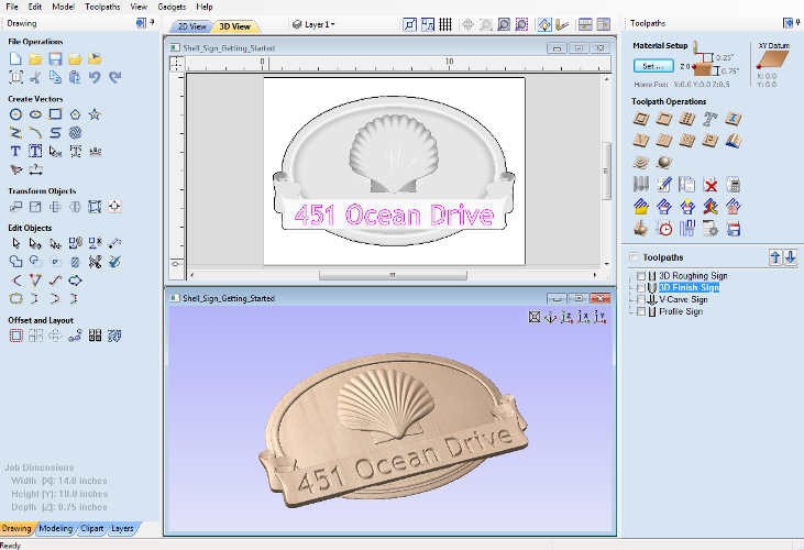
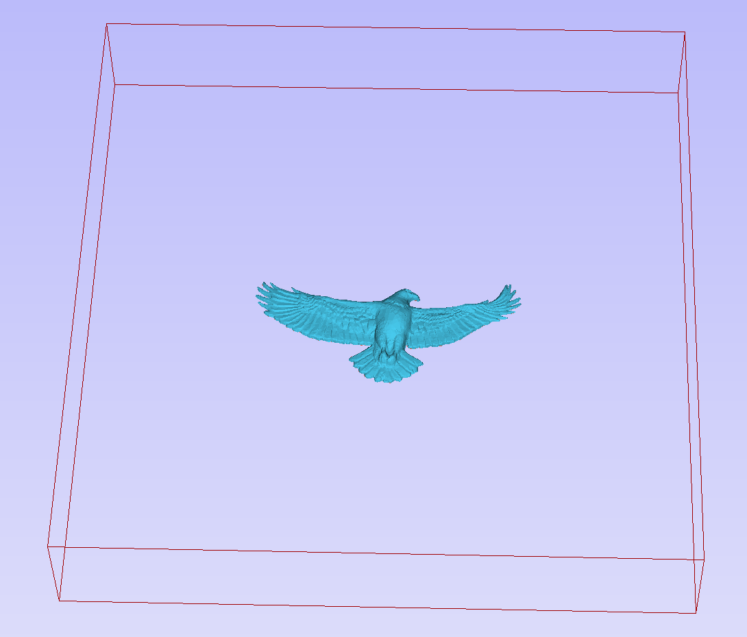
Aspirehas been designed to work in a way which enables the user to easily create even very complex projects. In any situation, the best approach to producing something complicated is to break it down into smaller pieces until a level of simplicity is reached that can be understood and managed. In Aspirethis is achieved by letting the user work with pieces of the design which are combined to make the finished part. In the terminology of the software these pieces are called Components. To help organize the Components they are assigned to Levels. Step by step, Components and Levels can be created and modified until you have all the elements you need. In the images below you can see an example of how this might work. On the left you can see the separate component for a model of a bunch of grapes and on the right you can see these positioned to make the complete part - we call this resulting combination the Composite Model.
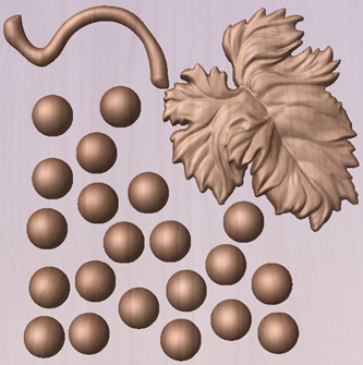
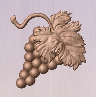
There is no limit to how simple or complex a Component or the Components on a Level can be (this is the user's choice). In the example shown, you can see that a model of a whole bunch of grapes may be made up of smaller individual components but they could also be combined to exist as one single Component (the assembled bunch of grapes) that could then be used to lay-out a more complex part with multiple bunches of grapes. They could also be organized so all the grapes were on one Level and leaf and stem on another to provide a different way of managing and manipulating the shapes. Each user will find a level of using Components and Levels they are comfortable with which may be dependent on the particular job or level of proficiency with the modeling tools.
3D Components and Levels
In Aspire, the aim is to end up with a set of Components and Levels that when combined together will make the finished 3D part. One way to think of this is like building a 3D collage or assembly. As the design evolves, new Levels or shapes may need to be created or existing ones changed. The parts of the collage are managed with the Component Tree which will be covered in more detail later.
Creating and Editing Components
An existing Component can be copied, scaled and have other edits carried out on it as an object. The user can also change the way it relates to the other Components, for instance whether it sits on top or blends into an overlapping area of another Component. The shape, location and relation of these pieces determine the look of the final part. As the job progresses, the user will need to create brand new Components or edit existing ones by adding new shapes, combining them with others or sculpting them.
Components can be created and edited by:
- Use a modeling tool to create shapes from 2D vectors.
- Import a pre-created 3d model - either a model previously created in Aspire or from another source such as a clipart library or a different modeling package.
- Create a 'texture' Component from a bitmap image.
- Use the Split Components Tool to break an existing Component into multiple pieces.
All of these methods are covered in detail throughout the training material.
Dynamic Properties
As well as having its underlying 3D shape, each component also has a number of dynamic properties that can be freely modified without permanently changing its true shape. These include scaling of the Component's height, the ability to tilt it, or to apply a graduated fade across it.
These dynamic properties can always be reset or altered at any time during your modeling process, which makes them a particularly useful way of 'tweaking 'your components as you combine them together to form your final composite model.
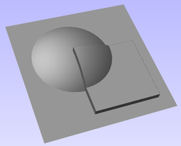
Combine Modes
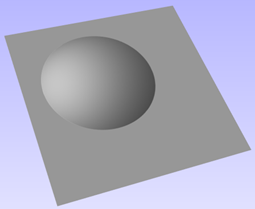
The Combine Mode is a very important concept when working with 3D shapes within Aspire. The options for combine mode are presented when creating new shapes and also when deciding how Components and Levels will interact in the Component List. Rather than cover this in every section where it is applicable, it is worth summarizing the options here so the general concept can be understood.
When you have more than one 3D shape, such as the Component pieces of the design or where you have an existing shape and are creating a new one, then you need to have a way to tell the software how the additional entities will interact with the first. This can be an abstract concept for users who are new to 3D but it is an important one to grasp as early as possible. In Aspire this is controlled by a choice called the Combine Mode.
There are four options for this: Add, Subtract, Merge High, Merge Low.
As modeling is an artistic and creative process, there is no general rule to describe when to use each one. As a guide though you can assume that if the second shape's area is completely within the originals one then you will probably be adding or subtracting and if the shapes only partly overlap that you will probably use Merge or, very occasionally, Low.
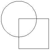
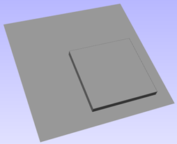
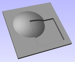
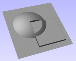
The four options and their specific effects are described on the following pages. To illustrate the different effects a combination of an overlapping beveled square and a dome will be used. You can see in the image top right how these are arranged in the 2D View and how they overlap. Then you can see each individual shape in the images below middle and right. These shapes will be used to demonstrate the different Combine Modes. In every case the Dome will be considered the primary shape and the square is the secondary shape which is being combined with the first. In addition to the dome/square example some images of 'real world' parts will also be included to help to understand how these can be used on actual projects.
As well as working on individual shapes, the Combine Modes are also assigned to Levels. These will govern how the combination of all the individual components on one Level interacts with the result of all the Components on the Level below it in the Component Tree
Note:
There is a 5th Combine Mode available from the right mouse click menu after a component has been created called Multiply. This combine mode has specialist applications which are dealt with in the appropriate tutorial videos. This option will literally multiply the heights of the Component or Levels being combined to create the new Composite 3D shape.
Add
When Add is selected, it takes the first shape and then just adds the height of the second shape directly on top of the first. Any areas which overlap will create a shape which is exactly the height of each shape at that point added together (see below)
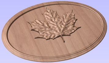
Typically the add option is mainly used when the shape being added sits completely within the original shape, this ensures that the uneven transition where the parts only partly overlap (as shown in the example) do not occur.
The example above shows the Maple Leaf and border extrusion Components being Added to the dome Component in the sign example from the Introduction to Modeling document.
Subtract
When Subtract is selected it takes the first shape and then removes the height of the second shape from the first. Any areas which overlap will be a combination of the original height/shape less the second shape. Areas where the shape goes into the background will become negative regions. You can see how this looks using the dome and square in the image below:
Typically subtract, like the add option, is mainly used when the shape being removed sits completely within the original shape, this ensures that the uneven transition where the parts only partly overlap (as shown in the example) do not occur.
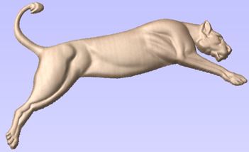
The image shown above has some 'creases' to help define the muscles of the lioness. The shapes to create these recesses were created by using the Subtract option with the Create Shape tool on the vectors representing those recessed areas.
Merge
When the Merge option is selected any areas of the shapes which do not overlap remain the same. The areas that overlap will blend into each other so that the highest areas of each are left visible. This results in the look of one shape merging into the other and is in effect a Boolean union operation. You can see how this looks using the dome and square in the image below:
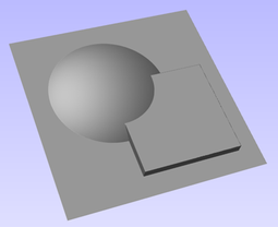
Typically the merge option is used when the shape being combined partly overlaps the original shape. This enables a reasonable transition to be made between them.
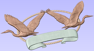
The image above shows 2 Herons, a rope border and banner Components. Each of these overlaps with the others and so they are set to Merge in this areas. Whatever is the higher of the two merged areas is what is prominent. In this case the rope is lower than everything and the Banner is higher than the Herons so the desired effect can be achieved.
Low
The Low option is only available when combining Components (not in the modeling tools). When this mode is selected, any areas which do not overlap are left as they were in the original two shapes. Any areas which overlap will create a new shape which is the lowest points taken from each shape, this is in effect a Boolean intersection operation. You can see how this looks using the dome and square in the image below:
The Low option is used for recessing a shape into a raised shape. An example of this is shown in the image above.
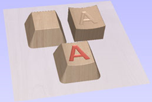
The example shown on the right above uses the Low option to combine the flat topped 'button' component on the left with the curved top face component with the letter 'A' on the right. Combining both components with the merge low option gives the keyboard button with the curved top you see in the bottom row.
Level Mirror Modes
Right-clicking Levels in the component tree will open a pop-up menu offering commands and operations related to the clicked level and Mirror Modes can be set in this way. If a mirror mode is set on a Level, all the components it contains will be continually mirrored dynamically as they are moved, transformed or edited. The mirroring is non-destructive, that is it can be turned off or on at any time and does not alter the underlying components in any permanent way. Working inside a Mirror modes Level is a simple way of achieving a complicated symmetrical pattern by editing only one half (or quarter, see below) of the design.
The available Mirror Modes are broadly divided into two groups. The first group apply one plane of symmetry:
- Left to Right
- Right to Left
- Top to Bottom
- Bottom to Top
These modes allow you to work in one half of your job and the other half will be automatically and dynamically generated for you. For example, in Left to Right mode you would place your components in the left half of your job and a mirrored equivalent of each would be created in the other half of the job. This 'reflection' is updated dynamically as you work.
The other group offer two planes of symmetry (horizontal and vertical):
- Top Left Quadrant
- Top Right Quadrant
- Bottom Left Quadrant
- Bottom Right Quadrant
When using these modes your components should all be in the quadrant (quarter) of the job. Mirrored reflections horizontally and vertically will be created in the other quadrants of the job for you.
Multi Sided View

When working in a 2 Sided environment you can create components independently per side or using the Right click option you can copy or move a component to the opposite side. Selecting the option to work in 'Multi Sided View' allows you to view components you may have on the Top and Bottom side in the 3D View. In the Toolpath Preview form of a project that contains toolpaths for the Top and Bottom Sides the multi sided view presents the simulation of the toolpath preview on both sides also, if the multi sided view is not selected you can use the 'Preview all Sides' option in the Toolpath Preview form to display the Top and Bottom Toolpaths in the 3D view. 2 Sided Setup will be described in detail later in the relevant section of this manual.
Archivos de trayectoria de herramienta 3D
Los archivos de Cut3D, PhotoVCarve y Design y Make Machinist de Vectric que incluyen trayectorias de herramienta 3D se pueden importar a Aspire mediante los comandos de menú principal: Archivo ► Importar ► PhotoVCarve, Machinist o Cut3D Toolpaths.
El archivo 3D primero debe escalarse al tamaño requerido antes de que se calculen las trayectorias de herramienta y, a continuación, el archivo completo guardado listo para importarlo a Aspire. Estos archivos solo se pueden mover y colocar dentro de Aspire, pero no se pueden escalar.
Se dibuja una miniatura en escala de grises del trabajo 3D en la vista 2D con el origen X0 Y0 en la posición en la que se estableció en Cut3D, PhotoVCarve o Design y Make Machinist. Las trayectorias de herramienta asociadas también se dibujan en la ventana 3D y los nombres aparecen en la lista Trayectoria de herramienta.
Posicionamiento
Para mover las trayectorias de herramienta de diseño 3D, abra la ventana 2D, haga clic en el ratón izquierdo dos veces en la imagen en escala de grises (se vuelve azul claro para indicar que está seleccionada) y, a continuación, arrastre a la posición deseada o utilice las herramientas Mover o Alineación para un posicionamiento preciso.
Las trayectorias de herramienta se mueven automáticamente en la ventana 3D a la misma posición XY que la imagen.
Las trayectorias de herramienta para el ejemplo anterior se han calculado con el X0 Y0 en el medio del diseño 3D. Cuando se importan a Cut2D, los datos se colocan automáticamente utilizando las mismas coordenadas, lo que coloca tres cuartas partes del diseño fuera del trabajo. En la segunda imagen, la imagen en escala de grises se ha movido al centro del trabajo.
Las herramientas de dibujo de simetría y rotación 2D también se pueden utilizar para editar el conjunto de datos 3D.
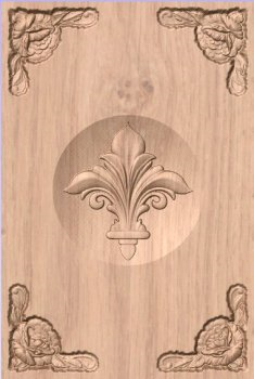
Las trayectorias de herramienta 3D también se pueden copiar mediante el comando Duplicar trayectoria de herramienta en la ficha Trayectorias de herramienta, lo que facilita el uso de varios elementos de un único diseño en un trabajo. La vista previa en miniatura también se copia para cada trayectoria de herramienta, lo que facilita la colocación de copias adicionales de una trayectoria de herramienta 3D.
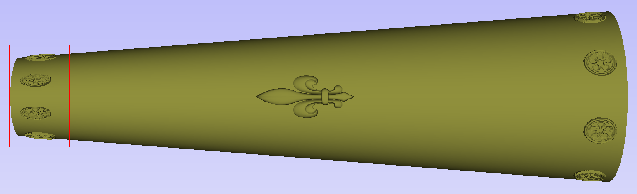
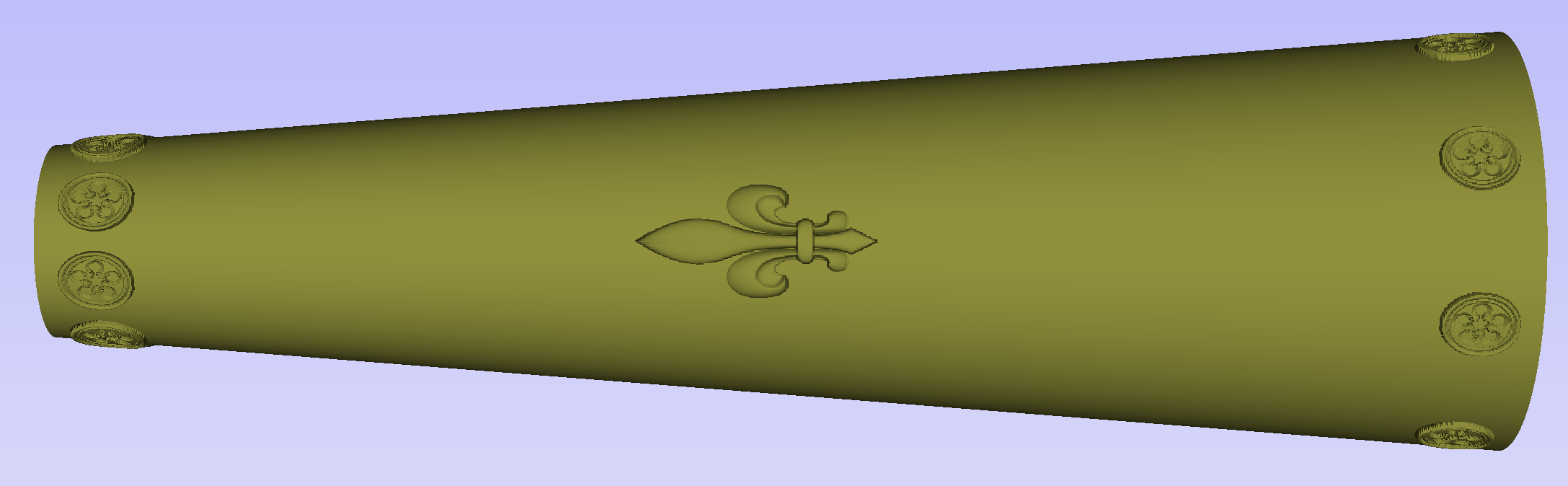
Por ejemplo, un solo diseño se puede copiar y reflejar para crear versiones izquierda y derecha de un diseño 3D o para colocar varias copias de un diseño decorativo en las esquinas de un panel de la puerta del gabinete como se muestra a continuación.
Las trayectorias de herramienta para los elementos 3D se pueden previsualizar junto con las trayectorias de herramienta convencionales Perfil, Bolsillo y Perforación, y todo se guardará listo para el mecanizado.
Un buen ejemplo de dónde se podría utilizar esta funcionalidad junto con PhotoVCarve es para hacer marcos de imagen personalizados que incluyen las ranuras de PhotoVCarve, además de texto grabado descriptivo y un borde decorativo perfilado o biselado. Como se muestra a continuación:


Opciones
Las trayectorias de herramienta importadas también se pueden editar para colocarlas dentro del material o para cambiar los parámetros de corte: las velocidades y las velocidades de avance se pueden cambiar.
Design and Make Machinist
Al utilizar un archivo Design and Make Machinist que incluya varias trayectorias de herramienta, debe recordar editar la Profundidad de inicio para todas las trayectorias de herramienta 3D importadas.
Haga clic en el icono Editar trayectoria de herramienta o haga doble clic en el nombre de la trayectoria de herramienta para abrir el formulario de edición.
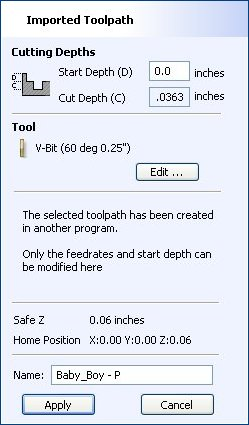
Por ejemplo, después de mecanizar un bolsillo de media pulgada de profundidad, se puede editar un diseño de PhotoVCarve para tener una Profundidad de inicio de 0,5 pulgadas y esto tallará la fotografía en la base de la superficie del bolsillo.
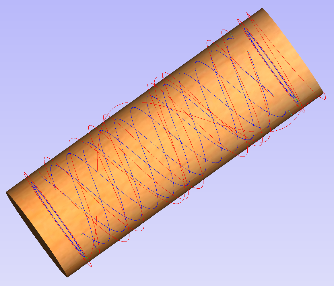
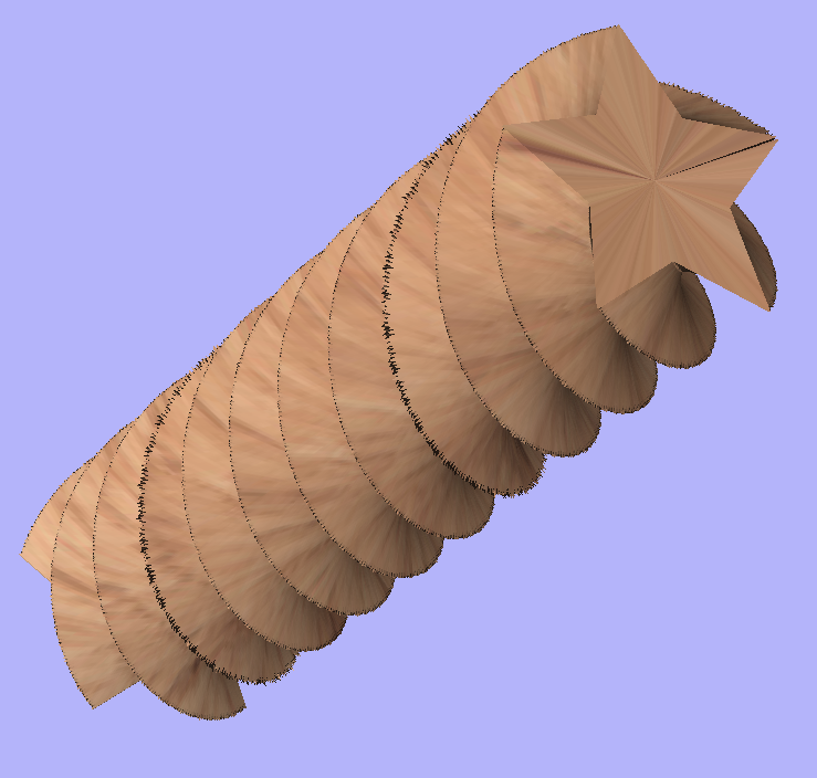
Rotary Machining and Wrapping
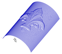
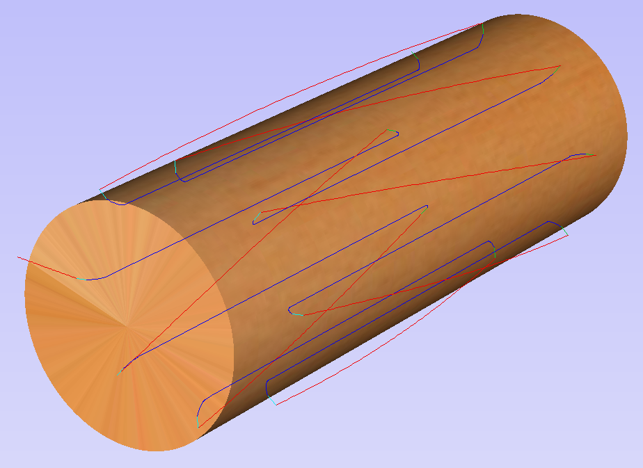
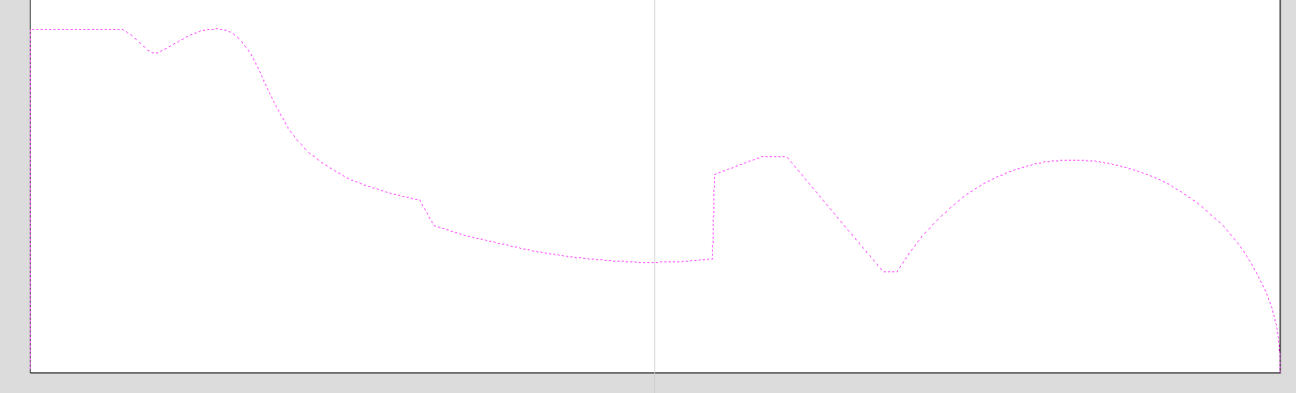
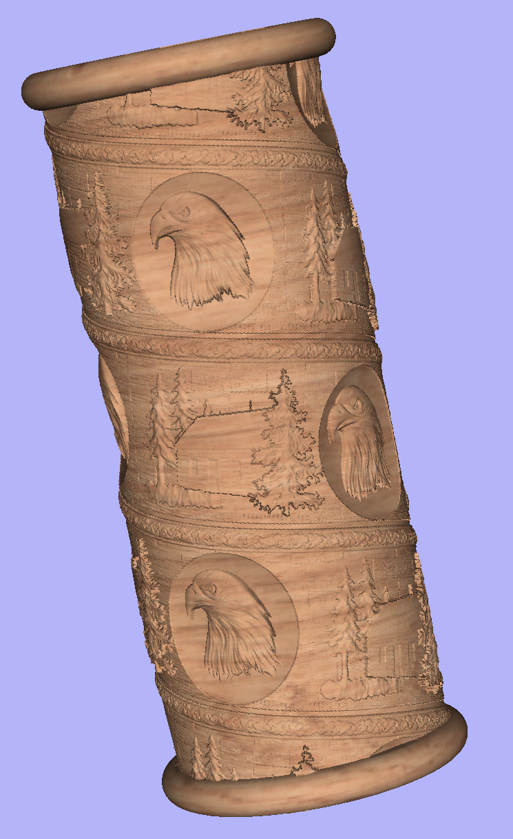
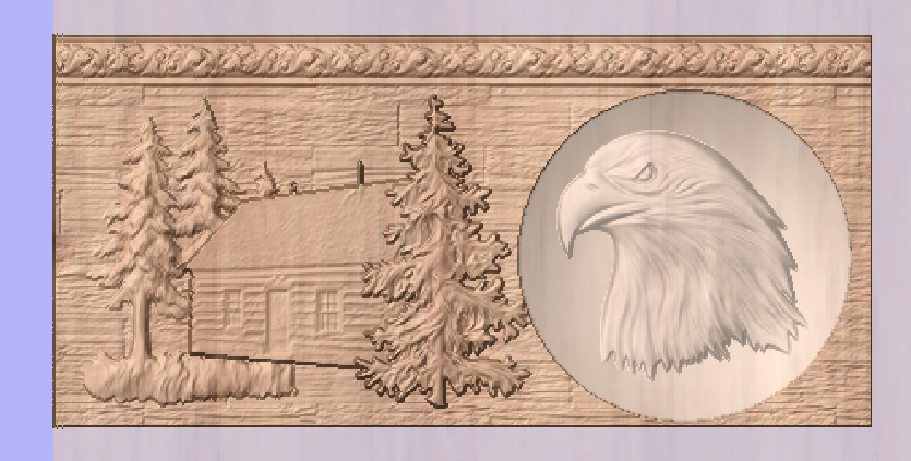
Aspire can 'wrap' flat toolpaths around a cylinder to provide output to CNC machines which are configured with a rotary axis / indexer. The image below shows a flat toolpath wrapped around part of a cylinder.
Note
It is important to note that wrapping works in conjunction with specially configured post-processors which take the XYZ 'flat' toolpaths and wrap them around a rotary axis, replacing either the X or Y moves with angular moves.
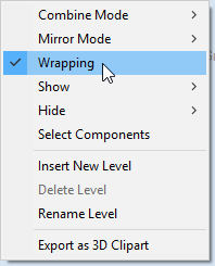
The toolpaths can be visualized wrapped within the program when the Auto Wrapping mode is on.
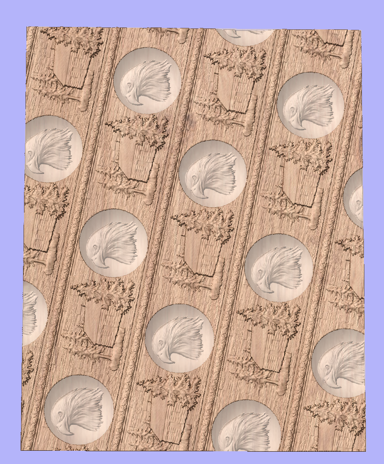
Aspire can also visualize a wrapped model within the program by drawing the shaded composite model wrapped.
Aspire also has the ability to draw the toolpath simulation wrapped. Although this is very useful for getting a feel for how the finished product will look, it is important to realize that the wrapped simulation may not be a 100% accurate representation of how the finished product will look. An example of potential difference would be if you drilled holes in your rotary job. In the actual work piece these will obviously just be round holes, in the wrapped simulation these may appear as distorted ovals due to the 'stretching' process which takes place when we wrap the flat simulation model for display.
Note
If your rotary axis is aligned along your Y axis you would choose the Orientation Along Y Axis option during job setup. All the examples in this document will assume that the rotary axis is aligned along X.
It is important to realize that there are a huge number of possible combinations of machine controller and axis orientations for rotary axis / indexers. This means it is impractical for Vectric to supply a pre-configured post-processor for every possible combination as standard. We include some wrapping post-processors in the default post-processor list as standard.
We also ship a copy of those post-processors in the Application Data Folder which can be accessed from the File Menu ► Open Application Data Folder.
The example below uses wrapped post-processors in sub-folder '05-Wrapped' under C:\ProgramData\Vectric\Aspire\V[ProductVersion]\PostP\05-Wrapped.
Examining these posts may be helpful if you need to configure a post of your own. If Vectric have not supplied as standard a post for your machine configuration please refer to the Post Processor Editing Guide accessible from the Help menu of the program for information on how to configure a post-processor and also look at the standard rotary posts Vectric supply.
You should also look at the Vectric forum to see if anyone else has already configured a post for your configuration or one similar. If, after looking at these resources you are still unsure of what needs to be done for your machine, please feel free to contact support@vectric.com for help. However, please note that we cannot guarantee to write a custom rotary post-processor for every individual requirement.
Creating a Rotary Job
XY Origin
XY Drawing Origin - Here you can specify where the XY zero origin will be placed on your job. These options correspond to the same fields on the normal 'Job Setup' form within the program. Most people would use the default Bottom Left Corner, but for some jobs you may prefer to have the XY origin in the Center.
- In a job with horizontal orientation (Along X Axis), the X offset will correspond to the length of the cylinder, and the Y offset will be a point along its circumference.
- In a job with vertical orientation (Along Y Axis), it's the opposite. The Y offset will correspond to the length of the cylinder, and the X offset will be a point along its circumference.
Orientation
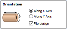
Cylinder Orientation Along - This section is used to tell the program how you have your rotary axis aligned on your machine. If you've already made your design, but just want to change the job for a different machine, then you could flip your design with the material so that all the vectors and components stay the same relative to the job.
Z Origin On - This section determines whether the Z Origin is set to the surface of the material or the base (center of cylinder). These settings can be over-ridden when the toolpath is actually saved, but we would strongly recommend the 'Cylinder Axis' is selected for rotary machining. The reasons for this are detailed in the note below.
Z Origin
You have the choice of specifying if the tool is being zeroed on the center of the cylinder or the surface. When you are rounding a blank, you cannot set the Z on the surface of the cylinder, as the surface it is referring to is the surface of the finished blank. We would strongly recommend for consistency and accuracy that you always choose 'Center of Cylinder' when outputting wrapped toolpaths as this should always remain constant irrespective of irregularities in the diameter of the piece you are machining or errors in getting your blank centered in your chuck.
Tip:
A useful tip for doing this is to accurately measure the distance between the center of your chuck and a convenient point such as the top of the chuck or part of your rotary axis mounting bracket. Write down this z-offset somewhere, and zero future tools at this point and enter your z-offset to get the position of the rotary axis center. Another reason for choosing 'Center of Cylinder' is that some controls will be able to work out the correct rotation speed for the rotary axis based on the distance from the center of rotation. If the Z value is relative to the surface, the control would need to know the diameter or radius of the cylinder at Z zero.
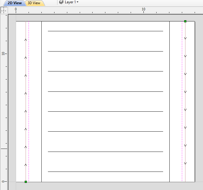
Vector Layout
As well as creating a job at a suitable size for wrapping toolpaths, when creating the job, it will create a number of vectors which can be very useful when creating your wrapped job.
The vectors are created on their own individual layers and by default these layers are switched off to avoid cluttering up your work area. To switch on the layers, display the 'Layer Control' dialog (Ctrl+ L is the shortcut to show / hide this). To show / hide the layer simply click on the check box next to the layer name.
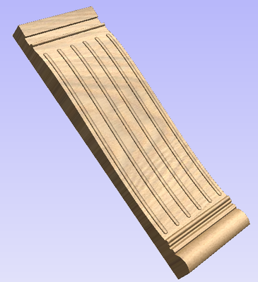
2Rail Sweep Rails - This layer contains two straight line vectors which can be used to sweep a profile along if you are creating a shaped column.
Bounding Box - This layer contains a rectangular vector covering the entire job area. This vector is useful if you are going to machine the complete surface of the cylinder.
Choosing stock material
When setting-up rotary project, software assumes a perfect cylinder with an exact diameter. In practice the stock material may be uneven, or only blank with square profile may be available. In those cases blank needs to be machined into cylinder of desired size, before running toolpaths associated with the actual design.
Another consideration is length of the stock material. Typically, part of the blank will be placed within the chuck. It is also important that during machining, the cutting tool is always in safe distance from both chuck and tailstock. For those reasons, the blank has to be longer than the actual design. When setting-up the machine for cutting, one has to pay extra attention to ensure that origin is set accordingly to avoid the tool running into chuck or tailstock!
If the design was created without those considerations in mind, the blank size can always be adjusted in the Job Setupform.
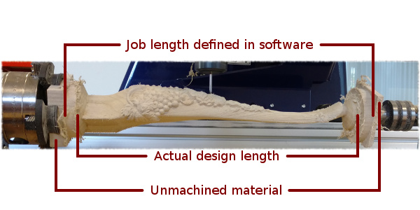
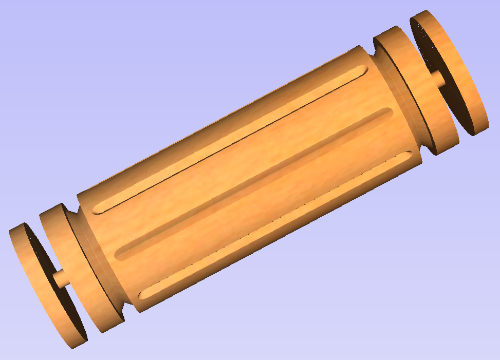
The picture below presents an example of a rotary project layout. As explained above, the actual blank is longer than job defined in Aspire to allow for the chuck and sufficient gaps. The actual design is shorter than job defined in Aspire, to leave some space for tabs, that can be machined with the profile toolpath prior to removing the finished part from the chuck.
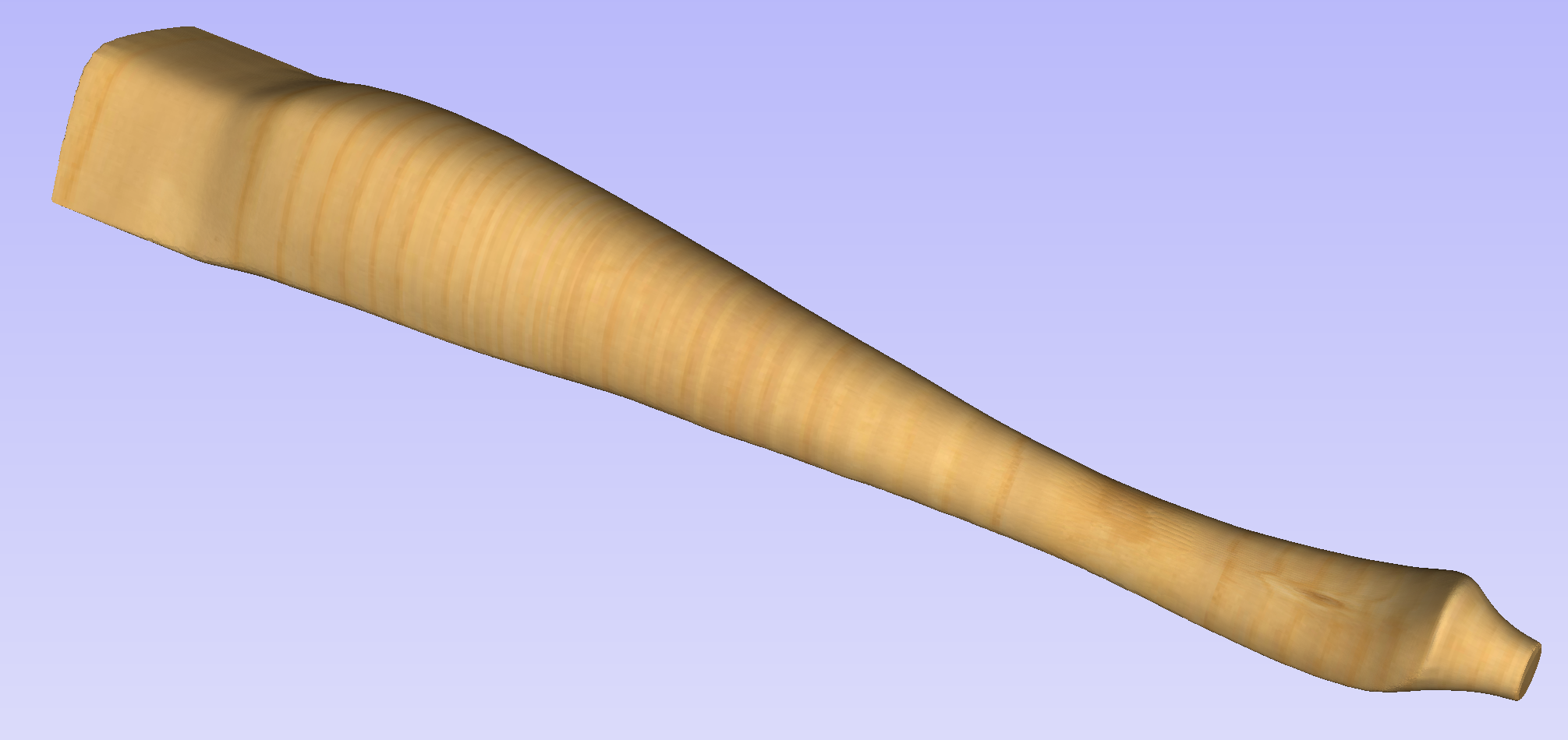
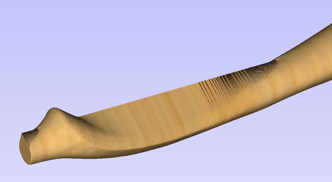
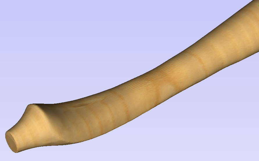
When machining 3D shapes with varying thicknesses like on the example shown below, it is a good idea to place the thicker end of the model on the side closest to the driving motor. This way torsional twisting will mostly affect the stronger end of the machined part and help to avoid bending or breaking of the part during machining.
Importing External Models in a Rotary Project
Importing Full-3D models
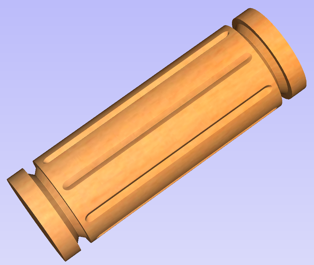
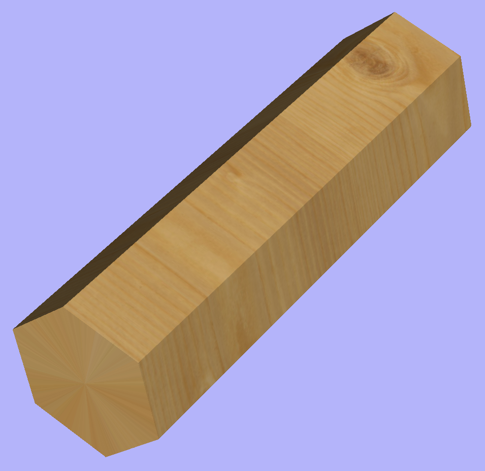
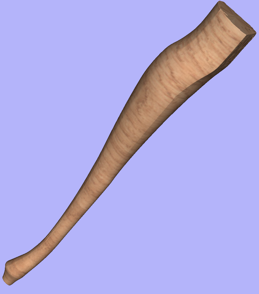
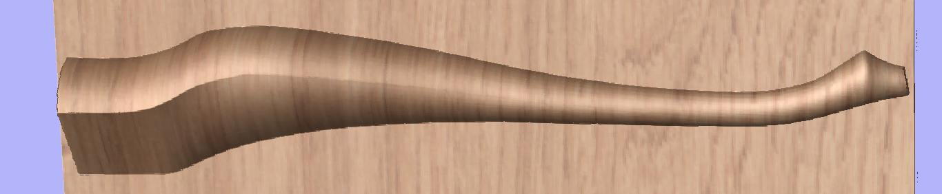
This section will present the process of importing the Full-3D STL model into rotary project, using a table leg as an example.
Overview
There are two basic use cases when importing an external model into the rotary job. The first case involves bringing a model designed for this particular job in another software. Thus the dimensions of the imported piece may already be correct and it can be desired to use them for the size of project. The second use case is when importing a stock model that would have to be scaled to fit on particular machine.
Aspire uses following workflow that covers both of those cases:
- Setting-up rotary project
- Choosing file for import
- Orientating the model in material block
- Scaling the model
- Finishing the import
Setting up a rotary project
Create a new job using the Job Setup form. It is important to set the job type as rotary to ensure a proper import tool is used in the next step.
If the dimensions of the project are already known, they could be specified directly.
If it is desired to fit the model to a given machine or stock available, set both the diameter and length to maximum. During import the model will be scaled to those limits.
If it is desired to use the imported model size, any size can be specified at this time. During the model import the project can be automatically resized to match the model dimensions.
In this example it was desired to fit the model into a specific stock size with a Diameter of 4 inches and a Length of 12 inches. XY origin was set to centre.
Importing the file and orientating it
To start the importing process, use Import a Component or 3D Model tool from the Modelling tab
Make sure that the Imported model type is set to Full 3D model .
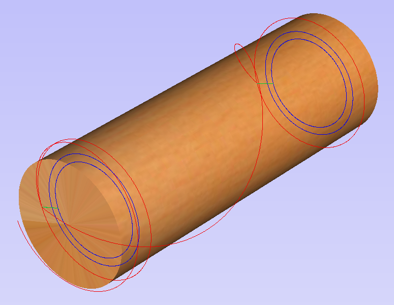
The first step is to position the imported model within the material. This step is necessary as this information is not present in the imported file. When the model was opened, the import tool chose the initial orientation, as can be seen below.
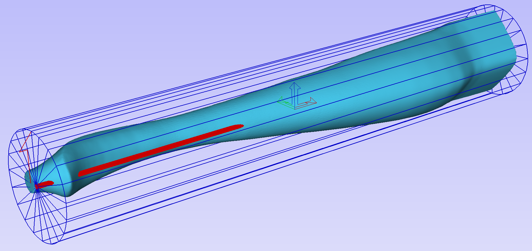
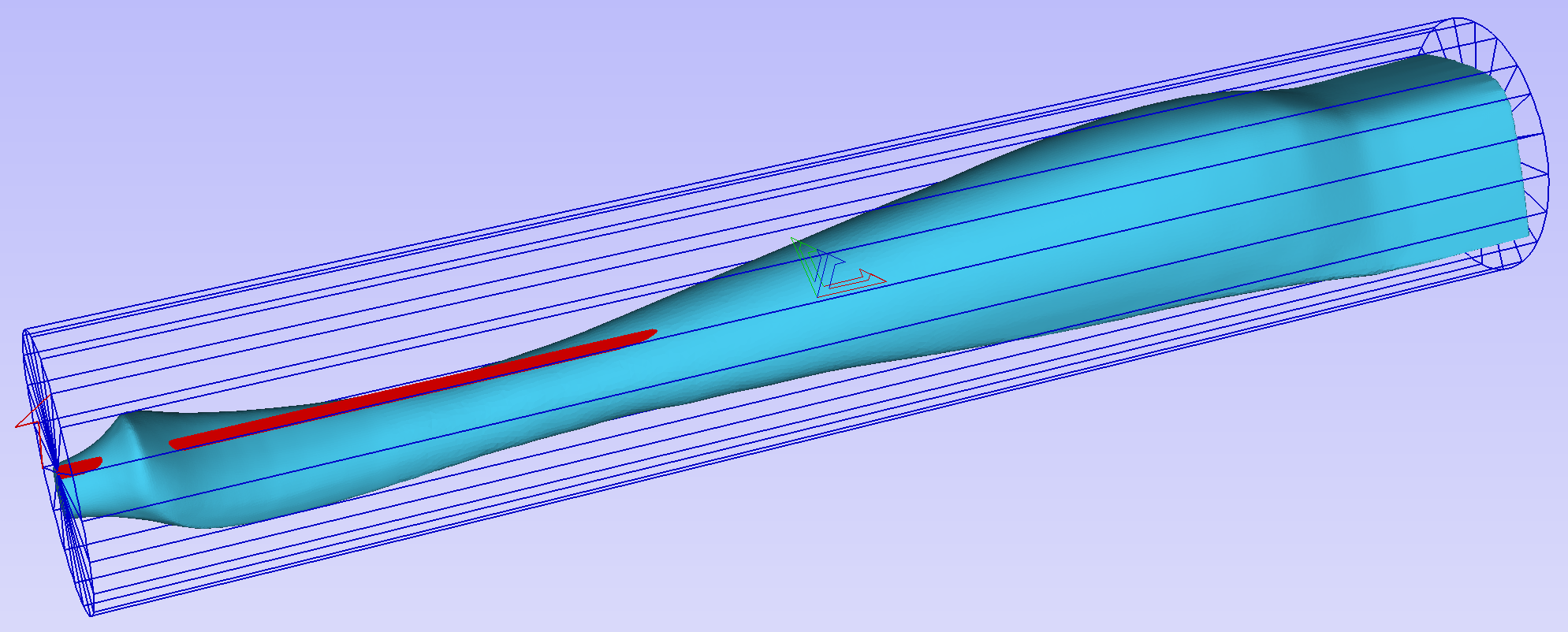
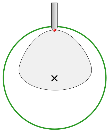
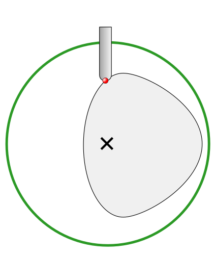
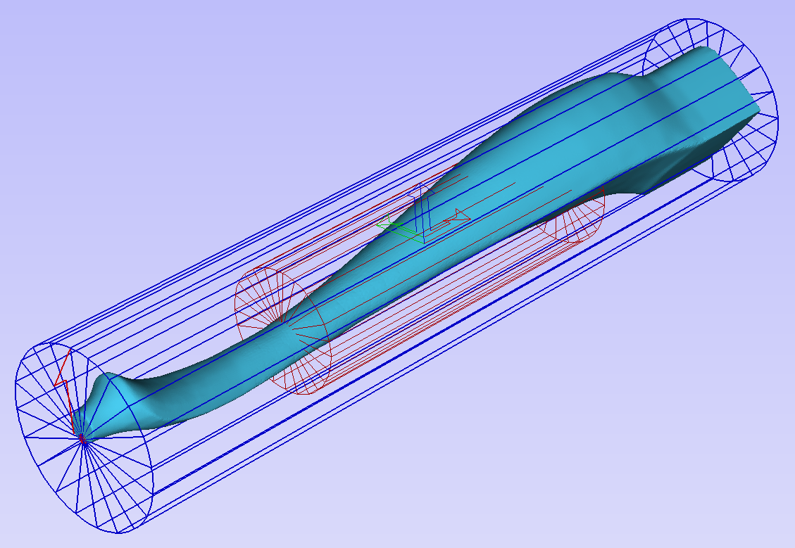
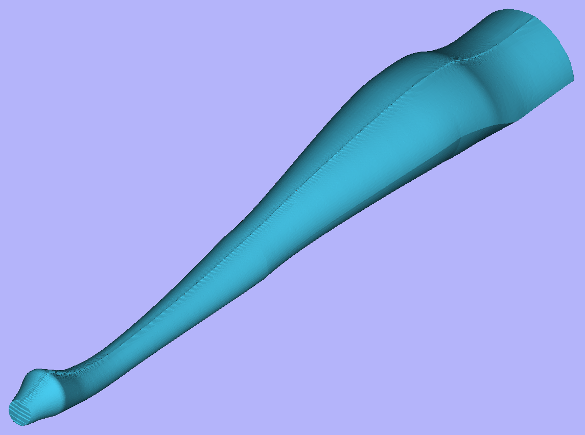
To help with orientating the model, the software displays a blue bounding cylinder. This cylinder has the rotation axis aligned with that defined for the material block and thus can be used as a reference. Its size is just big enough to contain the imported model at the current orientation. When the model orientation is changed, this blue cylinder will shrink or grow so it always contains the model. At this stage its exact dimensions are not important, as we are only interested in positioning the model correctly.
The software also highlights the rotation axis in red. This is particularly important when importing bended models. It is currently not possible to represent areas of model that are entirely below or above the rotation axis. This is the case in the example shown here. If the model was imported as is, the distortion would be created as can be seen below. Therefore it is important to position the model in a way such that the rotation axis is contained within the model.
The last guiding element displayed by the software is the red half arrow on the side of the cylinder. This arrow is indicating the position that corresponds to the center of the wrapped dimension in the 2D view. In this example the model is orientated in such a way, that front of the leg would be placed on side of the 2D view, rather than centre. Thus it is better to rotate model so this arrow points to the front of the imported model.
The import tool provides a few ways of adjusting the model orientation. The most basic one is the Initial Orientation. This can be used to roughly align the model with the rotation axis. This can also be combined with the Rotation about Z Axis.In this example the tool chose Left with no rotation. In order to align the front of the leg with the red arrow, one could use the Front and -90 as the Rotation about Z Axis.
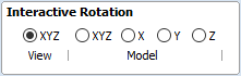
Once the initial orientation is decided, further adjustments can be made using the Interactive Rotation. The default option - XYZ View - disables the interactive rotation. That means that the 3D view can be twiddled with a mouse. Selecting other options enables the rotation around the specified axis.
In this example, instead of changing the initial orientation to align the front of the leg with the red arrow, one could select X Model option and rotate the piece manually. When selecting single axis rotation, the 3D view will be adjusted to show that axis pointing towards the screen. If any mistake is made, it is possible to undo rotation using Ctrl+ Z
Notice that whenever the part is rotated, it is always centered in the cylinder. In this example it is not desired, since we need the rotation axis to be contained within the model. In order to move the model in relation to the rotation axis, one can use the Rotation Axis Movement
Similarly to the previously described tool, when Rotation Axis Movement is set to Off, the 3D view can be panned
Correctly positioning the model for importing may require a combination of the Rotation Axis Movement and the Interactive Rotation to achieve desired results with models that bend. It is important to make sure that rotation axis is hidden in order to avoid distortion. However it is also desirable to have the rotation axis being in the center of each segment of the piece to ensure tool has angle close to the optimal during machining. Usually it is also useful to rotate the model in view around the axis after the adjustment, as this allows us to inspect the model from each side without the need to disable the Interactive Rotation before changing the viewing angle.
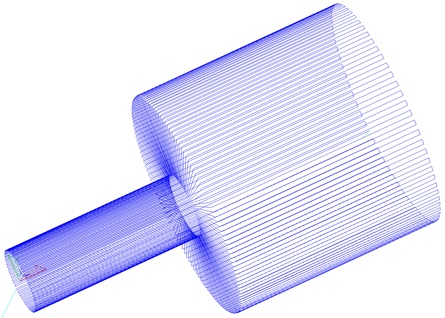
It is important to understand that Aspire does not support 4-axis machining. That means that while the machined piece can be rotated and tool moves along the rotation axis and in the Z direction, it is not possible to move the tool in the wrapped dimension and thus the tool is always above the rotation axis and cannot be moved to the side.
This limitation is shown below. The first picture presents correct machining of the point. If the tool moves to another location though, the angle will be incorrect and even worse, the tool side will be touching the stock.
Scaling imported model
Once model has been positioned as desired, its size can be taken into account.
By default the tool will assume that imported model is using the same units as the project. If that is not the case, model units can be switched. In this example project was set-up in inches, while imported model was designed in mm. After switching model becomes considerably smaller and a red cylinder, representing current material block is shown, as can be seen below.
At this point it is possible to specify the model size, in terms of diameter and length. This can be done manually by typing desired dimensions, or by fitting to material. If Lock ratio option is selected, the ratio between diameter and length is kept. One can also tick Resize material block option. If it is selected, the material block will be scaled to match current size of the model, after OK is clicked.
If it is desired to use model size as material block size, one can just make sure units are correct, then tick Resize material block option and press OK.
If it is desired for the model to fit material, one could click Scale model to fit material and tick Resize material block.
In this example model was fitted to material. Since in this case length of the piece is limiting factor and lock ratio is maintained, this results in model having considerably smaller diameter than material block. Hence Resize material block option was ticked.
Finishing import
After pressing OK the model will be imported as a component. It is possible to modify it as any other component or add pieces of decorative clipart onto its surface if desired.
It is important to keep in mind the distortion caused by the wrapping process. That means that wrapped toolpaths will match flat toolpaths only at the surface of the blank. The closer to the rotation axis (i.e. deeper) the toolpath is, the more it will be 'compressed'. This fact have a profound implication for 3D toolpaths. Consider the example shown below.
As can be seen if there is substantial difference in diameter in different parts of model, generating one 3D toolpath for whole model will result in wrapped toolpath being overly compressed. Thus it is usually better to create boundaries of regions with significantly different diameter and generate separate toolpaths using correct settings for each diameter.
Importing Flat Models
This section will present a process of importing Flat STL model into rotary project. Flat models are similar to decorative clipart pieces provided with Aspire and are supposed to be placed on the surface of modelled shape.
To start the importing process, use Import a Component or 3D Model tool from the Modelling tab
Make sure that Imported model type is set to Flat model
Again the first step is to select proper orientation of model. The tool will chose initial orientation and display model in the red material box. This box corresponds to the 'unwrapped' material block and its thickness is equal to half of the specified diameter of the blank.
If model is not oriented correctly, that is, does not lie flat on the bottom of the material box, as can be seen above, orientation have to be adjusted. To do that one can change Initial Orientation option and/or Rotation about Z Axis.
If the imported model is not aligned with any of the axes, it may be necessary to use Interactive Rotation. The default option - XYZ View - disables interactive rotation. That means that 3D view can be twiddled with a mouse. Selecting other options enables rotation around specified axis.
Each rotation can be undone by pressing Ctrl+ Z.
Once model is properly orientated, units conversion can be performed. By default the tool will assume that imported model is using the same units as the project. If that is not the case, model units can be switched.
There is also model scaling option included. When Lock ratio option is selected, the ratio between X, Y and Z lengths are kept. Note that once model is imported, it will be added to project as a component. Hence correct placement, rotation and sizing can be performed later, after model is imported.
If the project does not contain any models yet, following message will be displayed:
Typically you could simply click Yes.The more detailed explanation about modelling plane adjustment has been provided in Modelling 3D rotary projects
Simple Rotary Modelling using 2D Toolpaths
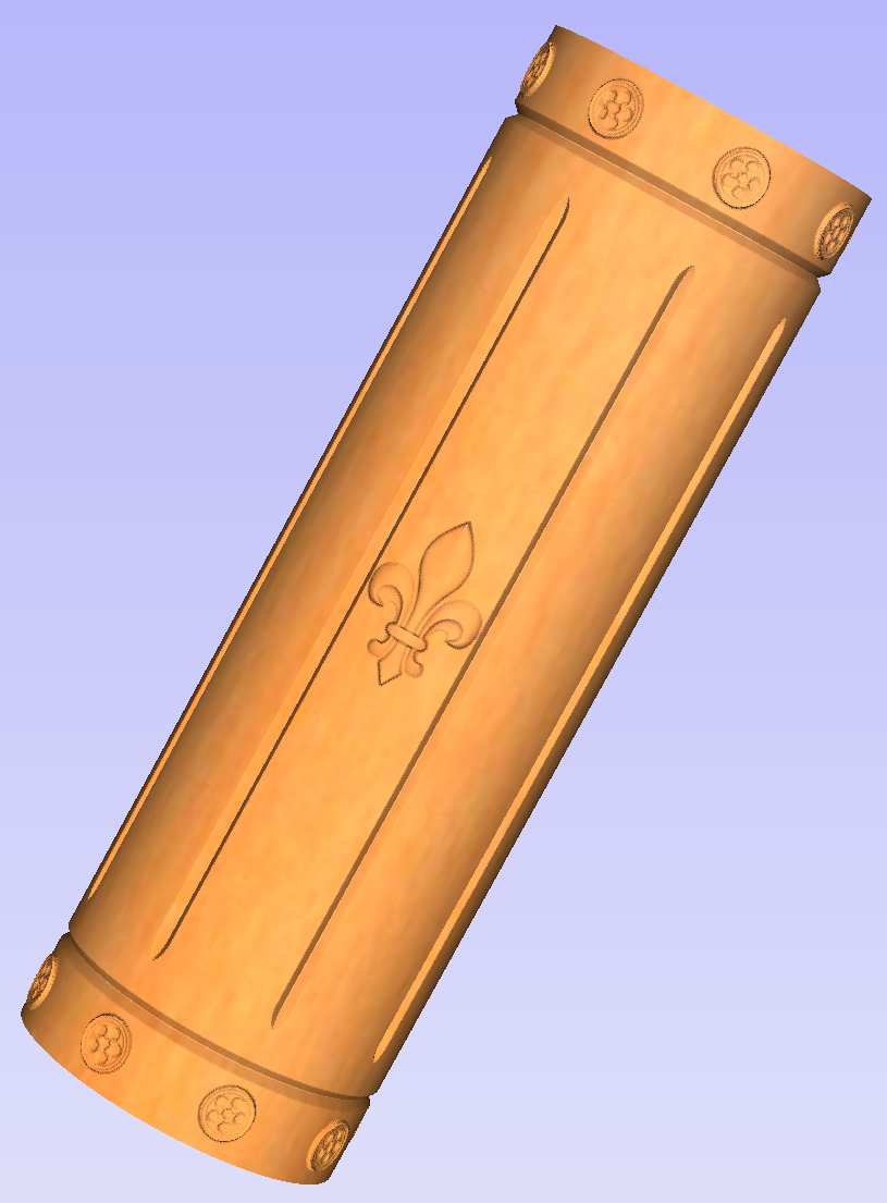
Creating vectors for a basic column
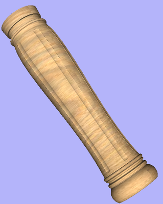
This section will show how to create a simple column, using the profile and fluting toolpaths.
Start by creating a new rotary job. Please note that settings shown here are only an example and should be adapted to match your machine setup and available material.
In this example the blank will rotate around X axis. We will refer to it as the rotation axis. The axis that will be wrapped is the Y axis. We will refer to it as the wrapped axis. That means that the top and bottom boundaries of the 2D workspace will actually coincide. We will refer to them as the wrapped boundaries.
First, create the cove vectors using Draw Line/Polyline tool. Those will run along the wrapped axis at both ends of the design. Snapping may be useful to ensure that the created line starts and ends at the wrapped boundaries.
In this example the coves were placed 1 inch from the job boundaries, leaving 10 inches in the middle for the flutes. The flutes will run along rotation axis. Assuming 0.5 inch gap between the cove and the beginning of the flute, the flutes will have the length of 9 inches. This example will use 8 flutes.
To start, create a line parallel to rotation axis that is 9 inches long. Now select the created flute vector and then select one of the cove vectors while holding down Shift. Then use Copy Along Vectors tool to create 9 copies. The original flute vector may now be removed as it is no longer necessary. Note that first and last copy are both created on wrapped boundaries. That means they will coincide, so one of them can be removed. As the last step select all flute vectors and press F9 to place them in the center of design.
Creating rotary toolpaths
The process of creating 2D rotary toolpaths is very similar to creating toolpaths for Single- and Double- models. This example will use the profile toolpath on the cove vectors. To create the toolpath, select the cove vectors and click on the Profile Toolpath from
To create the toolpath for the flutes, select the flute vectors and click on the Fluting Toolpath. This Example used a 1 inch 90deg V-Bit set to Flute Depth 0.2 and using the Ramp at Start and End and Ramp Type Smooth options. Ramp length was set to 0.25 inches. Both toolpaths can be seen below.
Simulating and saving toolpaths
It is time to simulate toolpaths using Preview Toolpaths. If the option to animate the preview is selected, the simulation will be visualized in flat mode. Once the simulation is complete, the wrapped rotary view will be turned back on automatically.
Contrary to single- and double- sided simulation, rotary simulation is not 100% accurate. For example round holes will appear in rotary view as oval ones, but obviously will be round when part is actually machined.
Although the design can be considered to be finished, in practice it is useful to be able to cut-out the remaining stock. This can be realized by making the design slightly longer and adding profile cuts. In this example the blank length was extended by 2 inches using the Job Setup . Existing vectors can be recentered using F9. After that the existing toolpaths have to be recalculated.
The cut-out vectors can be created in the same way as cove vectors. Two extra profiling toolpaths can be created using the suitable End Mill. In this example we used a tab with a 0.5 inch diameter. In order to achieve that, the user can type the following in the Cut Depth box: z-0.25 and then press = and the software will substitute the result of the calculation. Variable 'z' used in the formula will be substituted by the radius of the blank automatically by software. It is also important to specify Machine Vectors Outside/Right or Machine Vectors Inside/Left as appropriate. Cutout toolpaths and the resulting simulation has been shown below.
The final step is to save the toolpaths in a format acceptable by your machine. Use the Save Toolpaths and select the wrapped post-processor matching your machine.
Note
Tools and values presented in this example are for illustrative purposes only. Size of tools, feed rate, tabs diameter etc. have to be adapted to the material and machine used to ensure safe and accurate machining.
Spiral toolpaths
This section will explain how to create and simulate spiral toolpaths.
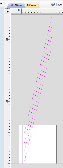
One way of thinking about spiral toolpaths is to imagine a long, narrow strip of fabric. Such a strip can be wrapped around a roll at a certain angle. In order to create a toolpath that wraps around the blank multiple times, one can create a long vector at a certain angle. Such a vector is an equivalent to the strip of fabric when it is unwrapped from the roll.
Although such a toolpath will exceed the 2D workspace of the rotary job, thanks to the wrapping process during both simulation and machining the toolpath will actually stay within material boundaries.
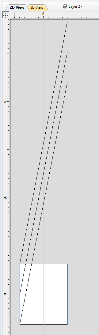
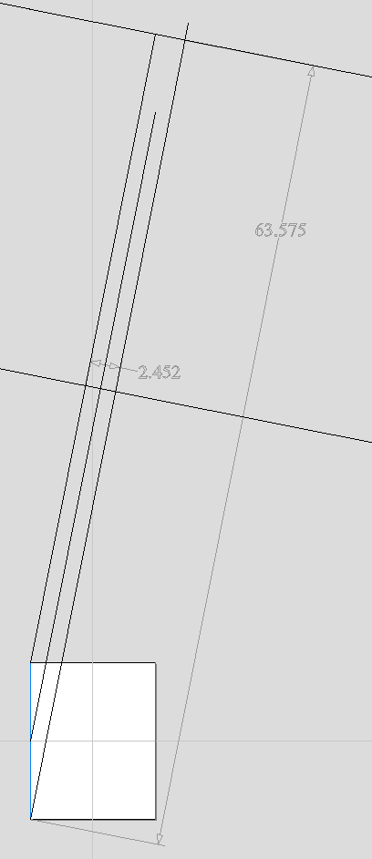
The most crucial part of designing spiral vectors is to determine the right angle and length of the line that would result in a given number of wraps. Suppose one would like to modify a simple column design to use spiral flutes, rather than parallel to rotation axis. The following example will use flutes wrapping 3 times each, but the method can be adapted to any other number.
All but one of the existing flute vectors can be removed. Select the Draw Line/Polyline and start a new line by clicking at one end of the existing flute. This line needs to be made along the wrapped axis with the length being 3 times the circumference of the job. In this example that means typing 90 into the Angle box and typing y * 3 into the Length box and pressing =. If the wrapped axis is not the Y axis, but rather the X axis, then the above formula should be x * 3.
Now one can simply draw a line connecting to the other end of the original flute vector and the newly created one. Using Copy Along Vectors tool this single flute may be copied in the way described earlier. In this example 4 spiral flutes were created, as can be seen below.
Once the flute vectors are ready, the toolpath can be created again using the Fluting Toolpath. An important thing to note, is the difference between the appearance of spiral toolpaths in the wrapped and flat view. By clicking on Auto Wrapping one can switch from wrapped rotary view to flat view and back again.
As can be seen above, in the flat view the toolpaths will follow the vectors and extend beyond the job boundaries. On the other hand the wrapped view, presented below, will display the toolpaths spiralling around the blank.
This was just a brief overview of general 2D workflow for rotary machining. Remember to also take a look at video tutorials dedicated to rotary machining, which are accessible from the Tutorial Video Browser link when the application first starts.
Modelling 3D Rotary Projects
Elaborating 2D designs with 3D clipart pieces
This section will present how to add 3D clipart to basic fluted column presented in Simple rotary modelling using 2D toolpaths.
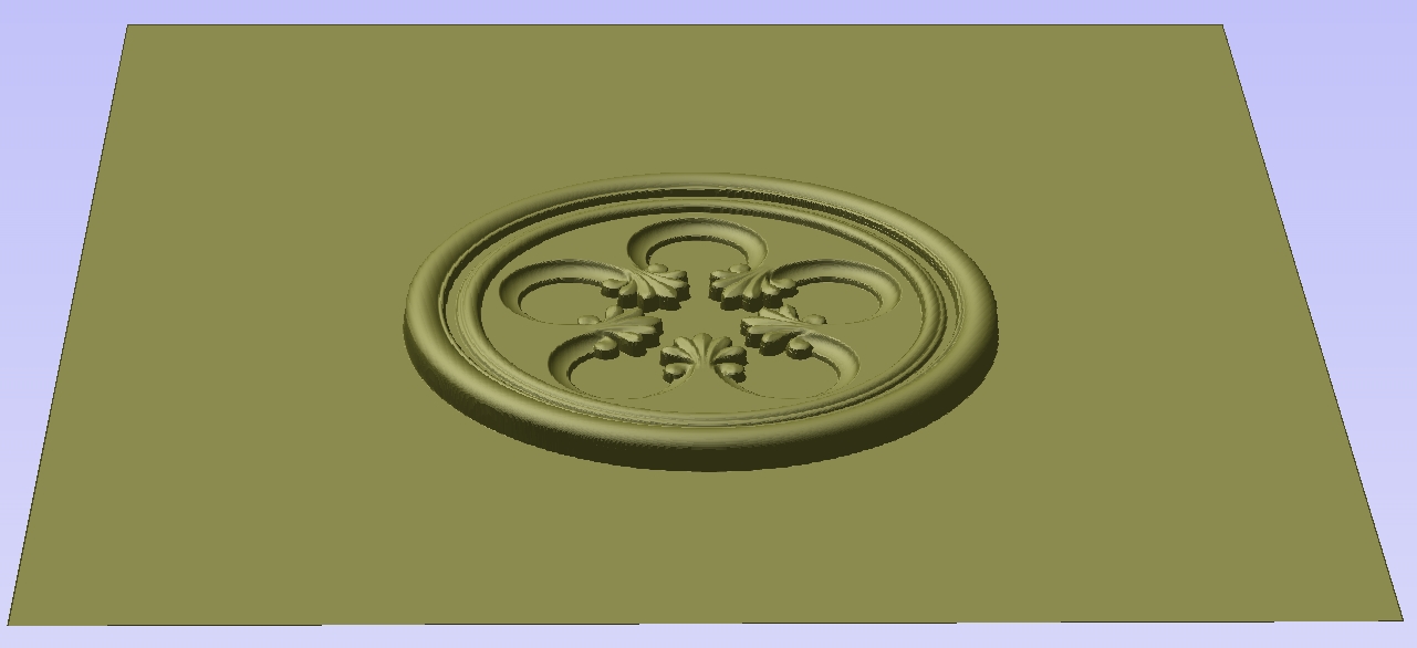
A simple way to start with 3D rotary models is to use add pieces of decorative clipart that is provided with Aspire. This process is very similar to adding clipart to single- or double- sided project, however there are some additional considerations that are specific to wrapped rotary machining.
To start, switch to the Clipart tab. Then choose a piece of clipart and drag and drop it into the workspace. Aspire will show following message:

To understand this message, we need to consider the flat view of our model, after importing the clipart. Flat view can be accessed by clicking Auto Wrapping button.
As can be seen, the model contains only the selected decorative piece on the flat plane. Although the column is obviously a cylindrical solid, so far we only used 2D toolpaths to carve details on the surface of cylinder. So the fact that machined piece is a cylindrical solid, derives only from fact that the blank is a cylindrical solid itself. Aspire allows the 3D model to also describe a solid body.
In this example the intent is to only place a decorative piece on the surface, rather than define body of the column. Aspire can see that we did not model a body and we are placing a piece of clipart, that is likely to be placed at the surface. By responding 'Yes' to the message we can confirm that it is our intent to use the component to decorate a surface.
Note
The above message is only displayed when the 3D model is empty. Regardless of user choice, this message will not be displayed again for this project.
More clipart can be placed as desired. Then the 3D view can be inspected. Once design is finished it is time to create toolpaths. In order to create 3D roughing toolpath, use 3D Rough Toolpath. Then create 3D finishing toolpath, using 3D Finish Toolpath. Select settings that are most appropriate for given application, while remembering which axis is rotating. The choice of axis may be particularly important if rotation axis speed is slower than linear axis.
In this example the decorative clipart that was added was not recessed. That means that after 3D machining the flat areas around clipart will be recessed due to clipart 'standing out' of the flat surface. Therefore existing 2D toolpaths needs to be projected. This can be accomplished by selecting Project toolpath onto 3D model option and recalculating the toolpaths.
Making a tapered column
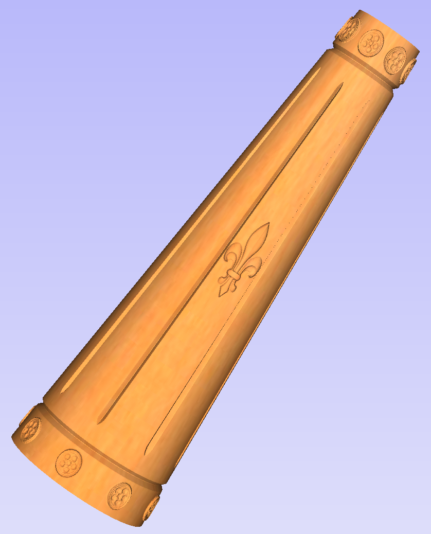
This section will explain how to make a tapered column by modifying the basic design from previous section.
So far only the surface details were modelled. In order to make a tapered shape, we need to model 'body' of the shape in addition to surface details. For that purpose, zero plane component can be used. It is added automatically for rotary jobs.
Double-click zero plane component to open Component Properties. Enter 0.8 in the Base Height box. Select Tilt option. Click Set button in Tilt section, then switch to 2D view and then click in the middle left and then in the middle right. Set angle to 3 degrees.
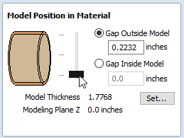
Since the modelling plane was adjusted for placing component on the surface, it needs to be adjusted again, so the component body is not 'inflated'. To do that open Material Setup form. Adjust modelling plane by moving slider down, until Gap Inside Model is 0.
After modelling a tapered shape, the 3D model of column will have a desired shape. However clipart pieces in the narrower parts have been distorted, as can be seen below. To fix that, one need to stretch the components in the wrapped dimension, to compensate for distortion.
The distortion that has been demonstrated above, applies also to toolpaths. That means that wrapped toolpaths will match flat toolpaths only at the surface of the blank. The closer to the rotation axis (i.e. deeper) the toolpath is, the more it will be 'compressed'. This fact have a profound implication for 3D toolpaths. Consider the example shown below.
As can be seen if there is substantial difference in diameter in different parts of model, generating one 3D toolpath for whole model will result in wrapped toolpath being overly compressed. Thus it is usually better to create boundaries of regions with significantly different diameter and generate separate toolpaths using correct settings for each diameter.
Modelling turned shapes
This section will present a basic technique for creating turned shapes.
Modelling turned shapes is quite easy. It requires a vector representing a profile of the desired shape and a Two Rail Sweep tool.
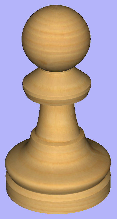
To start, create a new rotary job. Then either draw a profile using available drawing tools or import profile vector. This example used a chess pawn profile, as can be seen below.
Open the Two Rail Sweep tool. When the rotary job is created, the software inserts a special layer called '2Rail Sweep Rails'. It contains two blue lines on the sides of the job, that are perpendicular to the rotation axis.
Select both of those rails and click Use Selection button. The rails will be highlighted. Then select the profile vector and click apply. Inspect the 3D view to verify the results.
Modelling cross section
This section will explain how to model desired shape using Vector Unwrapper.
Vector Unwrapper is useful when rather than modelling a profile along the rotation axis, it is more intuitive to specify desired cross section. The tool transforms a vector, representing a cross section, into a profile vector that can be subsequently used with Two Rail Sweep tool.
Suppose we would like to create a hexagonal-shaped column. Let's start by creating a new rotary job. In this example job has a diameter of 6 inches and is 20 inches long. X axis is the rotation axis and Z origin has been placed on the cylinder axis.
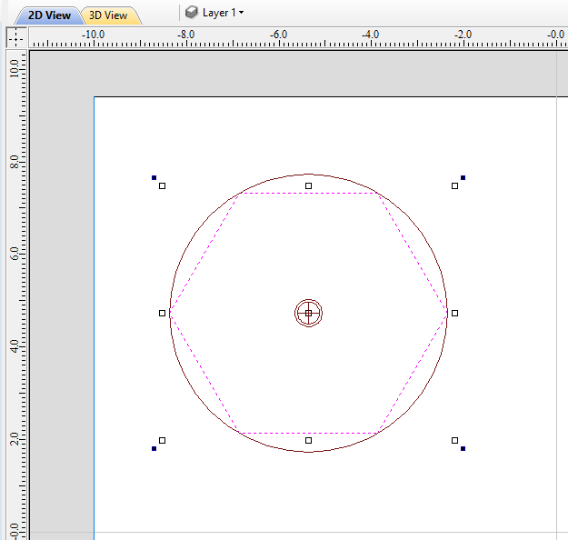
We need to create a hexagon using Draw Polygon tool. This vector will serve as a cross section and can be placed anywhere in the 2D view. In this example the material block diameter is 6 inches, so the radius of the shape cannot exceed 3 inches.
When the shape is created, select it and open Vector Unwrapper. The tool will display a cross hair in place where the rotation axis is crossing the profile and a circle with the diameter of the material block. This will help you determine whether the shape with such cross profile will fit in current material block.
In this example, Use Center of contour option was used. That means that rotation axis will be placed in the centre of vector's bounding box. One can also tick Simplify unwrapped vectors option to fit bezier curves, instead of using series of very short line segments. After apply is pressed, the unwrapped version of the selected cross section will be created, as have been shown below.
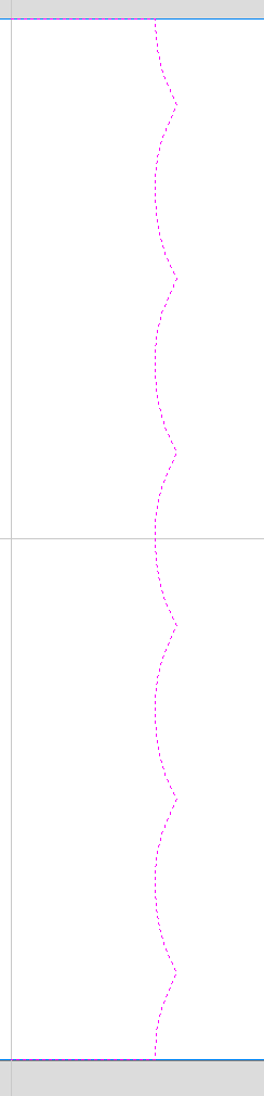
This example shows the unwrapped vector for a cylinder rotating around the X axis. If your rotary axis is aligned along Y the unwrapped vector will be horizontal. It is worth noting that unwrapped profile have 'legs' on each end. Those are needed to ensure that correct height will be used in the next step.
The tool automatically creates layer called 'Unwrapped Vectors Drive Rails' on which it places two blue line vectors on job sides, parallel to the rotation axis. In order to extrude the profile, open the Two Rail Sweep tool. Then select top and then bottom rail (left and right when Y axis is rotation axis) and confirm selection by clicking Use Selection button. Rails will become highlighted. Now click on unwrapped vector and press apply. The 3D view will show a hexagonal column, that can be seen at the beginning of this section.
Modeling Plane
The desired cross-section will only be achieved if modelling plane is positioned in cylinder centre. That means that Gap Inside Model is reported as 0 in Material Setup form. Otherwise the resulting model will have incorrect diameter and the cross section will become rounded.
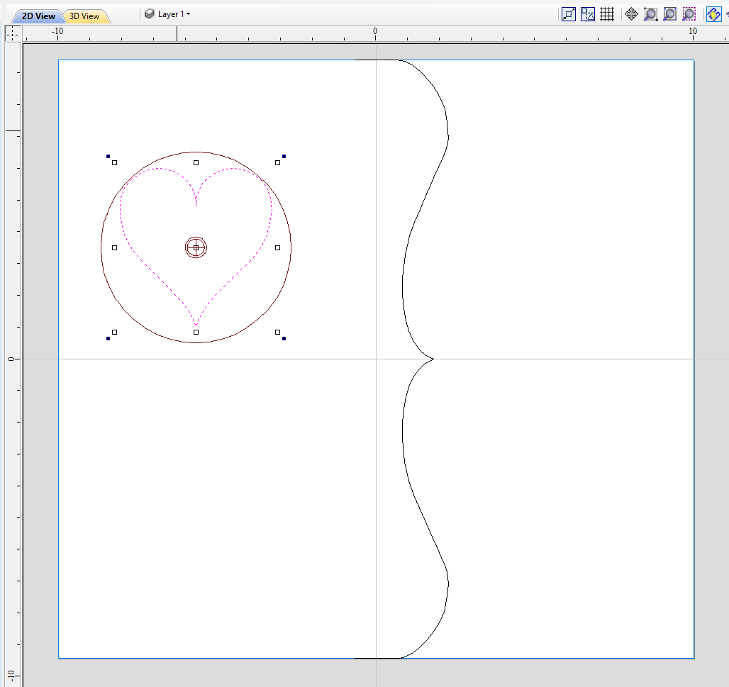
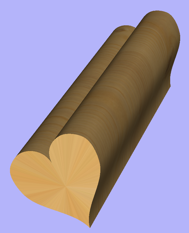
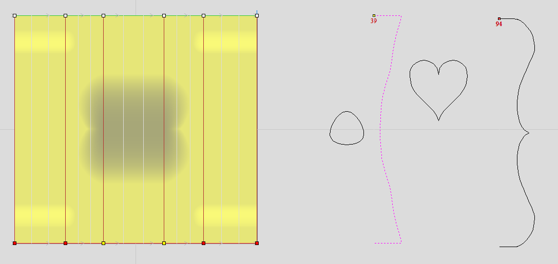
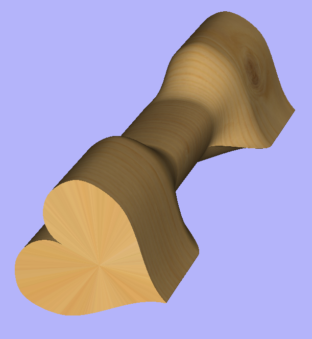
Vector unwrapper is not restricted to simple shapes. In principle it is always possible to use convex shapes and certain concave shapes. The example below shows a heart profile unwrapped.
If cross section in question is concave, one could imagine straight line starting in the center of the shape and touching a point on the boundary. If the second points keeps travelling along the boundary and each line is not crossing another point on the boundary, then it is possible to use this cross section. If the line does cross more than one point on the boundary, this part of the cross section will not be represented correctly.
All the examples so far used a single cross section. However it is also possible to use multiple cross sections.
Let's take another cross section and open Vector Unwrapper. Then drag the rotation axis handle a bit down from the center. If snapping is enabled, it can be used to help position the rotation center, as can be seen below.
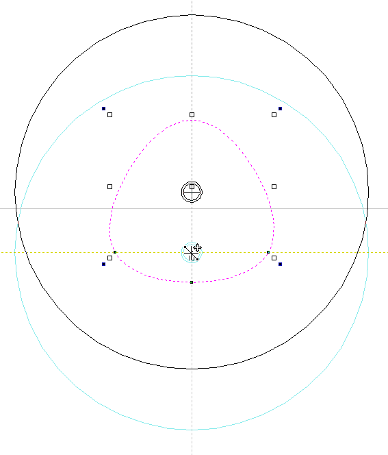
Once we have another unwrapped cross section, it is possible to use both during Two Rail Sweep. For example unwrapped heart profile can be placed twice on the left and twice on the right. The second unwrapped profile can be placed twice in the middle. Such arrangement may result in shape morphing, as can be seen below.
Advanced Modelling of 3D Rotary Projects
Modelling 3D spiral features
In this section we will show how to use level-wrapping feature to wrap a design in spiral manner around a column.
The workflow for creating spiral toolpaths has been presented in Simple rotary modelling using 2D toolpaths chapter. The basic idea involved creating a line at a proper angle to the rotation axis, that exceeded the 2D boundaries. When 2D toolpath is created based on such a line, it will be wrapped around material cylinder, creating a spiral.
This guide will build on that basic idea. The task is to create a horizontal strip with desired pattern and then wrap it like a ribbon around the cylinder.
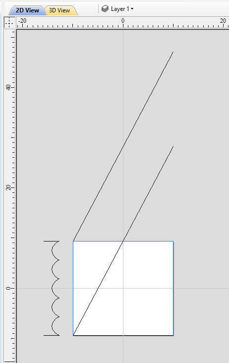
To help with that task, it is important to create some helpful vectors first. We need to create lines, that will become boundaries of our strip. In this example the strip was being wrapped four times around full length of material. This example assumes that rotation axis is parallel to X axis.
To start, select Draw Line/Polyline tool and draw a horizontal line at the bottom of the job from left to right. If it is desired for the spiral pattern to only fill part of the cylinder length, this horizontal line should be drawn only in th desired location. While the drawing tool is still active, type 90 into Angle box and type y * 4 into Length box and pressing =. We used y * 4 formula so the strip will wrap 4 times. Then press Add button to add a vertical segment.
Now, start a new line that connects the horizontal and vertical lines, forming a triangle. Once this line is created, horizontal and vertical lines can be removed.
The line that we just created will form a bottom of the strip. Now copy this line and place line so its bottom left end coincides with top left corner of 2D job. This line will form a top of the strip. Then make another copy and place it in the middle. This middle line will be used later to position our design within strip. All three lines have been shown below.
Next step is to find out the required length and width of the strip. We will need a few extra vectors to accomplish that.
Let's copy one of the created three lines and rotate by 90 degrees, to get a line that is perpendicular to the strip. Then place it in such way so it crosses the strip. This will help us measure the width.
Then copy the perpendicular line and place it so it touches the top line. Then extend the bottom line, until it crosses the perpendicular line we just added. This will help us measure the length of the strip.
Easiest way to achieve that, is to create a textured component. To do that, select the design in the component tree and activate the Create Texture Area tool. This example used the default settings of the tool. The tool will create a new component that will fill the whole 2D job boundaries. The component itself will be filled with the design in tiled manner. Now use Set Size tool to resize textured component to match the strip size.
Now the component have to be rotated and moved to fit between the lines be have drawn at the beginning. This process can be made easier by utilizing Copy Along Vectors tool. To proceed, activate the tool and select the textured component first, then select the middle line in the strip while holding Shift. Make sure that Align objects to curveoption is selected and use Number of copies option. Since our strip has already have a correct size, we only need one copy. However the tool would place the middle of our component at the beginning of the line only. If enter 3 as the number of copies, then the tool will place two copies of component at each end and in the middle. Afterwards copies at the ends can be simply deleted. The picture below shows the strip in the 3D view after being correctly positioned.
As can be seen, the strip disappears as soon as it leaves the material boundaries. In order to make it wrap around, we need to create a new level in the component tree and move the texture component into it. Then right click on the newly created level and right click. From the pop-up menu select wrapping. After that wrapping will occur.
Note:
Wrapping can be enabled on any level in component tree and combined with mirror mode. If the level wraps on itself, then intersecting areas will be merged regardless of level's combine mode. If it is desired to create e.g. a woven pattern, then place left-hand spiralled component and right-hand spiralled components in different separate levels, both with wrapping enabled.
The last step is to make column endings. For that purpose third level was created, with Combine Mode set to Merge. This way the spiral pattern will be 'hidden' at the ends. A circular 3D tab clipart was placed at each end, and stretch vertically to match the job boundaries.
Modelling twisted shapes
This section will show how to create twisted shapes, using combination of level-wrapping and Vector Unwrapper tool.
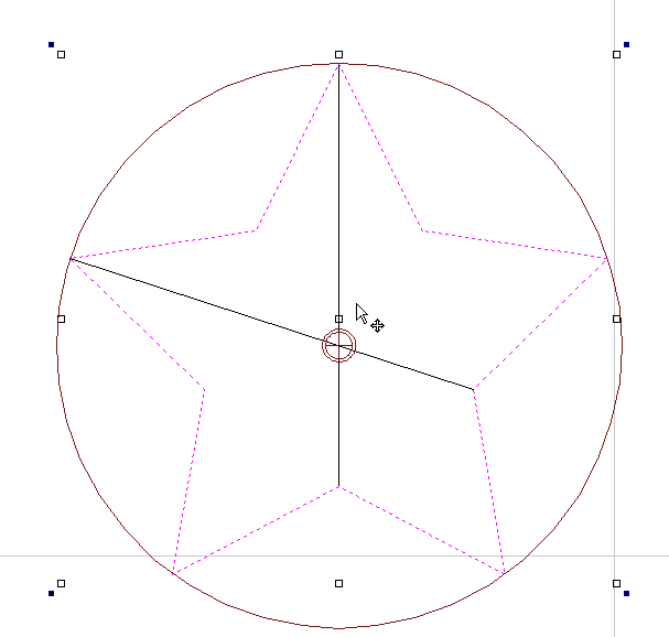
In this example a new rotary job was created, with diameter of 6 inches and length of 20 inches, rotating around X axis. To start, we need a cross-section vector. In this example a 5-armed star was used. To create a star, we can use Draw Star tool. This example used Outer Radius of 3 inches, to match the radius of the material.
The next step is to unwrap the cross section. In the case of star however, the center is not the same as center of star's bounding box. To find the real center, one can draw line from two of the star corners. Then open Vector Unwrapper and select the star. Then drag rotation center and snap it to the intersection of the lines, as can be seen below.
Once the star is unwrapped, we need to create rails, that will make spiral when wrapped. To do that, select Draw Line/Polyline tool and draw a horizontal line at the bottom of the job from left to right. While the drawing tool is still active, type 90 into Angle box and type y * 2 into Length box and pressing =. We used y * 2 formula so the star will make 2 revolutions Then press Add button to add a vertical segment. Finally, start a new line that connects the horizontal and vertical lines, forming a triangle. Once this line is created, horizontal and vertical lines can be removed.
Next step is to copy the line and place it so its bottom left end coincides with top left corner of 2D job.
Once the the rails are ready, one could use a Two Rails Sweep tool. However, since rails exceeds the 2D job boundaries, the created sweep will be cropped as soon as those boundaries are exceeded.
To overcome that, select both rails, open Draw Rectangle tool and press Create. This will create a bounding box containing the rails. Now, write done the size of the box and save current project. Then create a new single-sided project with the slightly bigger than the bounding box. Use Import Vectors option from the main menu and select previously selected file. Now select the rails and press F9 to center them.
Now use Two Rail Sweep tool. When component is ready, save the file.
Now re-open the original rotary project. Use Import Component and select single-sided project created in the step above. Move the component to the desired location. Then, create new level, move the component there and enable wrapping.
Using single-sided modelling tools
This section will present how to use single-sided modelling techniques in rotary projects.
Users familiar with modelling techniques used in single-sided projects may find them more convenient for modelling certain shapes. This example uses two vectors, representing side cross section of the table leg and a few of half cross sections for different parts of the table leg. Those vectors are presented below.
One can simply treat side cross section as rails and use Two Rail Sweep tool, placing half cross sections at appropriate locations. This way half of the leg can be modelled very quickly, with the result that can be seen below (using flat 3D view).
In order to use the created model in rotary project, we need to export and then import it back. Although it is possible to do this with two sessions of Aspire, it can also be done within a single session with rotary project. To export the leg model, make sure no other components are visible (including the automatically added zero plane) and open Export Model tool while holding down Shift. Pressing Shift allows to open the export tool in single-sided, rather than rotary mode.
Since half of the leg was modelled, Close with inverted front option was used. The resulting STL mesh can be seen below.
Once component is exported, it can be re-imported as Full 3D model. The model wil have a seam, in the place were two halfs were merged. This can be removed using smoothing function of Sculpting tool.
Edición de postprocesador
¿Qué hace el postprocesador?
El postprocesador es la sección del programa que convierte las coordenadas XYZ para que la herramienta se mueva a un formato adecuado para un router o máquina en particular. Este documento detalla cómo crear y editar los archivos de configuración que personalizan la salida del programa para adaptarse a un controlador de máquina determinado.
A continuación se muestran secciones de un programa típico que se ha procesado en G-Code y HPGL
Salida de código G
T1 M6
G17
G0 Z4.5000
G0 X0.0000 Y0.0000 S12000 M3
G0 X2.4567 Y7.8342 Z0.2500
G1 Z-0.0500 F5.0
G3 X3.3784 Y8.7559 I0.0000 J0.9218 F66.0
G3 X2.4567 Y9.6777 I-0.9218 J0.0000
G3 X1.5349 Y8.7559 I0.0000 J-0.9218
Salida HPGL
IN;PA;
PU2496,7960;
PD2496,7960;
AA2496,8896,90.000
AA2496,8896,90.000
AA2496,8896,90.000
AA2496,8896,90.000
PU2496,7960;
PU2496,6096;
Los fabricantes de controladores de máquinas a menudo personalizarán el formato de archivo necesario para que los programas se ejecuten en una máquina en particular con el fin de optimizar el control para adaptarse a las características individuales de esa máquina.
El postprocesador Vectric utiliza archivos de configuración basados en texto simple, para permitir al usuario adaptar un archivo de configuración, si así lo desea.
Secciones de postprocesador
Los postprocesadores Vectric se dividen en secciones para facilitar la claridad. Intente escribir sus postprocesadores en un estilo similar para facilitar la depuración.
Comentarios de archivo
Una sección en la que puede describir el postprocesador y registrar cualquier cambio en el postprocesador, cada línea es un comentario y comienza con un carácter '+' o un carácter ''.
+ Historial
+ Quién cuándo qué
+ ======== ========== ===========================
+ Tony 14/07/2006 Escrito
+ Marca 26/08/2008 Comandos ATC combinados, parada de husillo en TC
+================================================
Declaraciones de archivos globales
Las instrucciones son elementos que se usan solo una vez o tienen valores estáticos en todo el archivo. Escriba nombres de instrucción en mayúsculas para mayor claridad.
Statement | Result |
|---|---|
| The name that will appear in the post processor list |
| The file extension that the file will be given |
| The units that the file outputs (INCHES or MM) |
| The machine tool manufacturer has supplied a driver (usually a printer driver) thatn can directly accept the NC file output (For example see Generic HPCL_Arcs.pp) |
| Indicates that plunge moves to Plunge (Z2) height (that is set on the material setup form) are rapid moves |
| The control software uses a document interface that can directly accept the NC file output. |
| The moves in the Y axis are to be wrapped around a cylinder of the specified diameter. The "Y" values will be output as "A" |
| The moves in the X axis are to be wrapped around a cylinder of the specified diameter. The "X" values will be output as "B" |
| Spindle speed for this machine is output as a range of integer numbers between 1 and 15 representing the actual speed in RPM of the spindle, (between 4500 and 15000 RPM in the quoted example). For an example, see the file: Roland_MDX-40_mm.pp |
| This command allows you to substitute a character output within the variables (such as The characters are entered in pairs, Original - Subsititued. For example MACH 3 control software uses parentheses as comment delimiters, and does not allow nested comments. Most tools within the Vectric Tool Database have parentheses within the “Name” section; if these names are output, this would cause an error within Mach3. The command |
| Rotary: Enables / Disables output of the feedrate F in Inverse Time Feed Mode. In this mode, we're expected to complete a move in one divided by the F number of minutes. In GCode, this would G93 to switch on, or G94 to switch off and use units mode. |
Soporte para dividir cintas
Una sección que describe cómo se dividirá una salida de trayectoria de herramienta larga:
TAPE_SPLITTING=MAX_NUM_LINES LINE_TOL "FILENAME_FORMAT" START_INDEX INDEX_ON_FIRST_FILE
Por ejemplo, un comando de:
TAPLE_SPLITTING=1000 100 "%s_%s.tap" 1 "YES"
llevaría a...
La salida se dividirá en varios archivos de un máximo de 1000 líneas (+ por muchas líneas que haya dentro de la sección de pie de página del postprocesador), si existe un movimiento de retracto después de la línea 900 (1000 – 100), el archivo se dividirá en ese movimiento. Si el archivo se llamara "ruta de herramientas", los archivos divididos se denominarían toolpath_1.tap, toolpath_2.tap, etc. La primera salida de la trayectoria de herramienta será "toolpath_ 1.tap" no habrá ningún archivo llamado "toolpath" sin un número de índice, (como se utiliza INDEX_ON_FIRST_FILE= YES), a menos que el archivo tenga menos de 1000 líneas de largo, en cuyo caso el archivo no se dividiría.
Nota
Algunos controladores que requieren que los archivos NC se dividan, también tienen limitaciones en el número de caracteres dentro de un nombre de archivo. Por ejemplo, pueden requerir que el archivo se nombre con el formato de nombre de archivo 8.3 de estilo MSDOS. Esto debe tenerse en cuenta al asignar un nombre al archivo de salida.
Caracteres de terminación de línea
LINE_ENDING="[13][12]"
Valores decimales de los caracteres anexados a cada línea independiente del archivo postprocesado. (Por lo general será [13][10]) (Retorno de carro, avance de línea) para cualquier controlador que pueda leer un archivo de texto de formato MSDOS o Windows.
Numeración de bloques
Si desea agregar números de línea al archivo de salida, el número de línea actual se agrega con la variable [N]. El comportamiento de esta variable de número de línea se controla mediante las siguientes variables:
Statement | Result |
|---|---|
| Value at which the line numbering should start |
| Incremental value between line numbers |
| The maximum line number to output, before cycling to the Important - Some controllers have a limit to the number of lines that can be displayed on the control |
Variables
Variable Name | Output using | Value | Example File |
|---|---|---|---|
|
| Current Feed Rate. | Mach2_3_ATC_Arcs_inch.pp |
|
| Current Cut Feed Rate. | CNCShark-USB_Arcs_inch.pp |
|
| Current Plunge Feed Rate. | CNCShark-USB_Arcs_inch.pp |
|
| Current Spindle Speed in R.P.M. | GCode_arc_inch.pp |
|
| Current power setting for jet-based tools (e.g. lasers) | grbl_mm.pp |
|
| Current Tool Number. | Mach2_3_ATC_Arcs_inch.pp |
|
| Previous Tool Number. | NC-Easy.pp |
|
| Line Number. | Mach2_3_ATC_Arcs_inch.pp |
|
| Name of Current Tool. | MaxNC_inch.pp |
|
| Text from Note field in ToolDB for current tool | Busellato_Jet3006_arc_inch.pp |
|
| Name of Current Toolpath. | Viccam_ATC_Arcs_inch.pp |
|
| Filename (Produced by “Save Toolpath(s)”). | ez-Router_inch.pp |
|
| Folder Toolpath File was saved to. | Woodp_arc_mm.pp |
|
| Toolpath File Extension. | TekcelE_Arc_ATC_3D.pp |
|
| Toolpath Folder Pathname. | WinPC-NC_ATC_Arcs_mm.pp |
|
| Current coordinate of tool position in X axis. | GCode_arc_inch.pp |
|
| Current coordinate of tool position in Y axis. | GCode_arc_inch.pp |
|
| Current coordinate of tool position in Z axis. | GCode_arc_inch.pp |
|
| Current coordinate of tool position in A axis. | |
|
| Arc centre in X Axis (relative to last X,Y position). | Mach2_3_ATC_Arcs_inch.pp |
|
| Arc centre in Y Axis (relative to last X,Y position). | Mach2_3_ATC_Arcs_inch.pp |
|
| Arc centre in X Axis (absolute coordinates). | Isel_arc_mm.pp |
|
| Arc centre in Y Axis (absolute coordinates). | Isel_arc_mm.pp |
|
| Start position of an arc in X axis. | TextOutput_Arcs_mm.pp |
|
| Start position of an arc in Y axis. | TextOutput_Arcs_mm.pp |
|
| Mid-point of arc in X (absolute coordinates). | TextOutput_Arcs_mm.pp |
|
| Mid-point of arc in Y (absolute coordinates). | TextOutput_Arcs_mm.pp |
|
| Mid-point of arc in X (incremental coordinates). | TextOutput_Arcs_mm.pp |
|
| Mid-point of arc in Y (incremental coordinates). | TextOutput_Arcs_mm.pp |
|
| The radius of an arc. | Bosch_ATC_Arcs_mm.pp |
|
| The angle of an arc. | Generic HPGL_Arcs.pp |
|
| Home tool position for X axis. | CAMTech_CMC3_mm.pp |
|
| Home tool position for Y axis. | CAMTech_CMC3_mm.pp |
|
| Home tool position for Z axis. | CAMTech_CMC3_mm.pp |
|
| Safe Z Height / Rapid Clearance Gap. | EMC2 Arcs(inch)(*.ngc) |
|
| Diameter of cylinder that axis is wrapped around. | Mach2_3_WrapY2A_ATC_Arcs_mm.pp |
|
| Length of material in X. | Mach2_3_ATC_Arcs_inch.pp |
|
| Length of material in Y. | Mach2_3_ATC_Arcs_inch.pp |
|
| Length of material in Z. | Mach2_3_ATC_Arcs_inch.pp |
|
| Minimum value of material in X. | MaxNC_inch.pp |
|
| Minimum value of material in Y. | MaxNC_inch.pp |
|
| Minimum value of material in Z. | MaxNC_inch.pp |
|
| Maximum value of material in X. | MaxNC_inch.pp |
|
| Maximum value of material in Y. | MaxNC_inch.pp |
|
| Maximum value of material in Z. | MaxNC_inch.pp |
|
| Origin Position in X. | TextOutput_Arcs_mm.pp |
|
| Origin Position in Y. | TextOutput_Arcs_mm.pp |
|
| Z Zero Position, Table or Material Surface. | TextOutput_Arcs_mm.pp |
|
| X, Y Origin. | TextOutput_Arcs_mm.pp |
|
| List of tools used (In order of use). | Mach2_3_ATC_Arcs_inch.pp |
|
| List of toolpaths used in file (in order of use). | Mach2_3_ATC_Arcs_inch.pp |
|
| Toolpath Notes (Toolpath Control form). | Mach2_3_ATC_Arcs_inch.pp |
|
| File Notes (Edit > Notes). | Mach2_3_ATC_Arcs_inch.pp |
|
| File creation time. | Mach2_3_ATC_Arcs_inch.pp |
|
| File creation date. | Mach2_3_ATC_Arcs_inch.pp |
|
| Dwell time in seconds when drilling. | Mach2_3_Arcs_inch.pp |
|
| Name of the product used to output file, including version number. | |
|
| Tool diameter. | |
|
| Rotary: Current Inverse Time Rate | AvidCNC_WrapX2A_G93_inch.pp |
Formato de variables
Los valores de la posición de la herramienta, las velocidades de avance, las velocidades del husillo, etc., se insertan en el archivo utilizando variables. Las variables se utilizan en todo el archivo; las variables se reemplazan por el valor actual de ese elemento cuando se procesa el archivo. Por ejemplo, las posiciones actuales de las herramientas X, Y y Z en cualquier momento se insertan en el archivo utilizando la salida de la variable, [X], [Y] y [Z] respectivamente.
Escriba nombres de variables en mayúsculas para mayor claridad.
Una variable tiene el formato siguiente:
VAR VARIABLE = [VO|WO|CS|VF|MX]
Donde,
VO: salida de variable, por ejemplo X, XF o F.WO: cuando se emite, A=Siempre, C=Sólo cuando se cambia.CS: salida de cadena de caracteres antes del valor .VF: formato de valor, determina el formato con el que se genera el valor.MX: valor del multiplicador.
Una variable típica
1 | 2 | 3 | 4 | 5 | 6 | 7 | 8 | 9 | 10 | 11 | 12 | 13 | 14 | 15 |
|---|---|---|---|---|---|---|---|---|---|---|---|---|---|---|
|
|
|
|
|
|
|
|
|
|
|
|
|
|
|
VAR- Esta línea es una variable.- Nombre de la variable.
- Signo igual.
- Abrir corchete - (inicio de los parámetros de formato de variable).
- Etiqueta de variable - es decir, etiqueta que se sustituye por el valor de la variable.
- Barra vertical - Separador de parámetros.
A= Valor de salida siempre,C= Sólo valor de salida cuando cambia- Barra vertical - Separador de parámetros.
- Cadena de caracteres para imprimir antes del valor de la variable.
- Barra vertical - Separador de parámetros.
- Indicadores de formato opcionales - para obtener más información, consulte a continuación.
- Formato de valor - unidades y número de decimales para la salida.
- Barra vertical - Separador de parámetros.
- Multiplicador de salida - para obtener más información, consulte a continuación.
- Cerrar corchete cuadrado - Fin de los parámetros de formato.
Formato del valor de salida
La cadena de formato de valores debe tener el siguiente formato:
FORMAT_FLAGS FIELD_WIDTH DECIMAL_SEPARATOR DECIMAL_PLACES
Los indicadores de formato son opcionales y solo son necesarios para un pequeño número de controladores que se describirán en breve.
Ancho de campo: El ancho del campo representa el número mínimo de caracteres que se generan. El ancho del campo se establece normalmente en "1" pues un valor mayor que 1 normalmente solo es necesario si un controlador espera ver un número fijo de caracteres para el valor. Si este es el caso, se puede introducir un número mayor que 1. El número introducido garantizará que se genere el número de caracteres. El número que representa el ancho del campo incluye el número de punto flotante completo para el valor de salida (incluido el carácter separador decimal).
Separador decimal: El carácter separador decimal es casi siempre un carácter de punto, pero hay algunos controladores que esperan ver un carácter de coma. (Para ver un ejemplo de un postprocesador que no utiliza un carácter de punto, consulte el archivo: Heidenhain_inch.pp)
Decimales: El número de decimales de la salida posteriores al separador decimal. Los valores se establecen a menudo en 3 para los controladores que operan en sistema métrico, o 4 para los controladores que operan en pulgadas.
Indicadores de formato opcionales
Los valores de salida se pueden modificar aún más mediante los indicadores de formato opcionales:
Flag | Function | Default (without flag) |
|---|---|---|
| Left Justify the output | Values are right justified |
| Prefix the value with '+' or '-' | Only negative values are prefixed |
| If value has fewer characters than the set minimum, the value is prefixed with zeroes | Values is prefixed with blanks spaces |
| Values is always output with a separator character ( in practive this would only change the output value if the value is set to output integer values only) | When output is set to integer only, separator charactor is not appended to value. |
Formato predeterminado para variables
La mayoría de las variables tienen un formato predeterminado; (se muestra a continuación) para establecer un formato diferente para una variable, introduzca la línea siguiente en su postprocesador y modifique los parámetros para adaptarse a su controlador.
Default | Example |
|---|---|
|
The line number will always be output. An 'N' character will be inserted before the line number. It will be output as an integer number |
|
The spindle speed will always be output. An 'S' character will be inserted before the value and it will be output as an integer number. |
|
The feed rate will be output with an F character before the value, and will only be output when it changes. The value will be output to 1 decimal place Note In this format string there is an option extra parameter. This is the value multiplier. |
VAR PLUNGE_RATE = [FP|A||1.0] |
The plunge rate will be output with an F character before the value, and will only be output when it changes. The value will be output to 1 decimal place. Note In this format string there is an option extra parameter. This is the value multiplier. |
|
The cut rate will be output with an F character before the value, and will only be output when it changes. The value will be output to 1 decimal place. Note In this format string there is an option extra parameter. This is the value multiplier. |
|
The position value will be output with an ‘X’ character before the value, the position will Always be output, and will be output to 3 decimal places, this would typically be suitable for a control that requires metric output. If you wished to output the values to 4 decimal places as would be more typical for a controller operating in inches. You would format the line as follows.
|
|
The home position value will be output with an ‘X’ character before the value, the position will Always be output, and will be output to 3 decimal places, this would typically be suitable for a control that requires metric output. If you wished to output the values to 4 decimal places as would be more typical for a controller operating in inches. You would format the line as follows.
|
|
The value will be output with an ‘X’ character before the value, the position will Always be output, and will be output to 3 decimal places, this would typically be suitable for a control that requires metric output. If you wished to output the values to 4 decimal places as would be more typical for a controller operating in inches. You would format the line as follows.
Note In this format string there is an option extra parameter. This is the value multiplier. |
|
The value will be output with an ‘Y’ character before the value, the value will Always be output, and will be output to 3 decimal places, this would typically be suitable for a control that requires metric output. If you wished to output the values to 4 decimal places as would be more typical for a controller operating in inches. You would format the line as follows.
|
|
The value will be output with a ‘J’ character before the value, the value will Always be output, and will be output to 3 decimal places, this would typically be suitable for a control that requires metric output. If you wished to output the values to 4 decimal places as would be more typical for a controller operating in inches. You would format the line as follows.
|
|
The value will be output with a ‘J’ character before the value, the value will Always be output, and will be output to 3 decimal places, this would typically be suitable for a control that requires metric output. If you wished to output the values to 4 decimal places as would be more typical for a controller operating in inches. You would format the line as follows.
Note In this format string there is an option extra parameter. This is the value multiplier. |
|
The value will be output with a ‘X’ character before the value, the value will Always be output, and will be output to 3 decimal places, this would typically be suitable for a control that requires metric output. If you wished to output the values to 4 decimal places as would be more typical for a controller operating in inches. You would format the line as follows.
|
|
The value will be output with a ‘R’ character before the value, the value will Always be output, and will be output to 3 decimal places, this would typically be suitable for a control that requires metric output. If you wished to output the values to 4 decimal places as would be more typical for a controller operating in inches. You would format the line as follows.
|
|
The value will be output with a ‘A’ character before the value, the value will Always be output, and will be output to 3 decimal places, this would typically be suitable for a control that requires metric output. If you wished to output the values to 4 decimal places as would be more typical for a controller operating in inches. You would format the line as follows.
|
|
The value will be output with an ‘X’ character before the value, the value will Always be output, and will be output to 3 decimal places. |
Valor multiplicador
El valor del multiplicador se utiliza para multiplicar el valor para generar un valor diferente. Las razones habituales para desear hacer esto son:
- Para convertir la salida predeterminada de un postprocesador de pulgadas, de pulgadas por minuto a pulgadas por segundo, (multiplicar por 0.01666).
- Para convertir la salida predeterminada de un postprocesador métrico, de mm por minuto a mm por segundo, (multiplicar por 0.0166).
- Para que los valores positivos sean negativos (y viceversa), (multiplicar por -1).
- Para convertir la salida de un ángulo de arco de radianes a grados, (multiplicar por 57.2957795).
- Para multiplicar o dividir por un factor fijo (es decir, producir un modelo a escala 1:4, multiplicar por 0,25)
Bloques de postprocesador
HEADER
+---------------------------------------------------
+ Salida de comandos al inicio del archivo
+---------------------------------------------------
begin HEADER
"Commands"
El encabezado es la ubicación de las instrucciones que se generan una vez, al principio del archivo, y son comandos modales de configuración general para el controlador.
Por ejemplo, el encabezado puede contener un comando para mostrar el nombre de archivo en el controlador y una serie de "Códigos G" para configurar la máquina, por ejemplo G20 para indicar al control que los movimientos están en pulgadas, o G21 para indicar al control que los movimientos están en milímetros.
Las variables que es interesante incluir dentro de la sección de encabezado, podrían incluir:
Información sobre el bloque de materiales
- Extensión mínima en X = [XMIN]
- Extensión mínima en Y = [YMIN]
- Extensión mínima en Z = [ZMIN]
- Extensión máxima en X = [XMAX]
- Extensión máxima en Y = [YMAX]
- Extensión máxima en Z = [ZMAX]
- Longitud del material en X = [XLENGTH]"
- Longitud del material en Y = [YLENGTH]"
- Profundidad del material en Z = [ZLENGTH]"
Información de la posición de inicio
- Inicio X = [XH]
- Inicio Y = [YH]
- Página de inicio Z = [ZH]
- Brecha de separación rápida o Z Segura = [SAFEZ]
Detalles de la primera herramienta que se va a utilizar
- Número de herramienta = [T]
- Nombre de la herramienta = [TOOLNAME]
Velocidades de corte iniciales
- Velocidad de alimentación utilizada para cortar y hundir en el material = [F]
- Velocidad de alimentación mientras la herramienta está cortando el material = [FC]
- Velocidad de alimentación mientras la herramienta se hunde en el material = [FP]
- Los valores reales dependen del conjunto de unidades (consulte Configuración global de archivos) Los valores predeterminados son MM/Minuto o Pulgadas/Minuto, pero la salida se puede cambiar para adaptarse estableciendo el formato "VAR FEED_RATE" adecuado.
Velocidad del husillo
- Velocidad del husillo = [S] R.P.M.
TOOLCHANGE
+---------------------------------------------------
+ Salida de comandos en el cambio de herramienta
+---------------------------------------------------
begin TOOLCHANGE
"Commands"
Comandos que se generan cuando se requiere un cambio de herramienta. Las variables y comandos que se pueden utilizar incluyen:
- Número de herramienta anterior = [TP]
- Número de herramienta = [T]
- Nombre de la herramienta = [TOOLNAME]
- Nombre de la trayectoria de herramienta = [TOOLPATH_NAME]
- Nombre de ruta de acceso de herramienta = [PATHNAME]
- Nombre de archivo de trayectoria de herramienta = [TP_FILENAME]
- Directorio de archivos de trayectoria de herramienta = [TP_DIR]
- Extensión de trayectoria de herramienta = [TP_EXT]
- Velocidad del husillo = [S] R.P.M.
- M3 M Código utilizado a menudo para encender el husillo (rotación en el sentido de la reloj).
- M5 M Código utilizado a menudo para apagar el husillo.
NEW_SEGMENT
+---------------------------------------------------
+ Salida de comandos para un nuevo segmento (nueva trayectoria de
+ herramienta con número de herramienta actual)
+---------------------------------------------------
begin NEW_SEGMENT
"Commands"
Para ver un ejemplo de una sección de NEW_SEGMENT, consulte el archivo: Mach2_3_ATC_Arcs_inch.pp
Los comandos se emiten cuando una nueva trayectoria de herramienta utiliza la herramienta seleccionada actualmente, pero quizás se requiere una velocidad de husillo diferente o la máquina requiere instrucciones adicionales.
No es necesario incluir los comandos que se utilizan en la sección NEW_SEGMENT en la sección TOOLCHANGE, ya que un cambio de herramienta también llamará automáticamente a las instrucciones de la sección NEW_SEGMENT.
Las variables que se utilizan comúnmente incluyen.
- Velocidad del husillo = [S] R.P.M.
- M3 M Código utilizado a menudo para encender el husillo (rotación en el sentido del reloj).
- M5 M Código utilizado a menudo para apagar el husillo.
INITIAL_RAPID_MOVE
+---------------------------------------------------
+ Salida de comandos para movimiento rápido inicial
+---------------------------------------------------
begin INITIAL_RAPID_MOVE
"Commands"
Para ver un ejemplo de una sección de INITIAL_RAPID_MOVE, consulte el archivo: Saom_OSAI_Arc_inch.pp
Los comandos que se generan cuando se realiza el primer movimiento rápido después del encabezado o un cambio de herramienta. Una Sección no utilizada para la mayoría de los mensajes, pero útil si el primer movimiento rápido, necesita generar información diferente a los movimientos rápidos subsiguientes. Esta sección a veces es necesaria para las variantes HPGL.
RAPID_MOVE
+---------------------------------------------------
+ Salida de comandos para movimientos rápidos.
+---------------------------------------------------
begin RAPID_MOVE
"Commands"
Comandos que se emiten cuando se requieren movimientos rápidos.
FIRST_FEED_MOVE
+---------------------------------------------------
+ Salida de comandos para el primer movimiento de velocidad de avance en una
+ serie de movimientos de alimentación.
+---------------------------------------------------
begin FIRST_FEED_MOVE
"Commands"
Esta sección se utiliza comúnmente cuando los controladores requieren que la velocidad de alimentación se establezca en el primer movimiento de alimentación, esta velocidad se utilizaría para los movimientos de corte posteriores.
Para ver un ejemplo de una sección de FIRST_FEED_MOVE, consulte el archivo: Axyz_Arcs_ATC_inch.pp
FEED_MOVE
+---------------------------------------------------
+ Salida de comandos para movimientos de velocidad de avance
+---------------------------------------------------
begin FEED_MOVE
"Commands"
Se utiliza para generar información necesaria en cada movimiento, o todos los movimientos de alimentación, excepto el primer movimiento de alimentación, si una sección FIRST_FEED_MOVE está presente dentro del postprocesador.
FIRST_CW_ARC_MOVE
+---------------------------------------------------
+ Salida de comandos para el primer movimiento de arco en sentido
+ horario en una serie de movimientos de arco cw
+---------------------------------------------------
begin FIRST_CW_ARC_MOVE
"Commands"
Similar a la sección FIRST_FEED_MOVE, pero para los segmentos de arco en el sentido de las agujas del reloj. Esta sección se utiliza comúnmente cuando los controladores requieren que la velocidad de avance se establezca para el primer segmento de arco, esta velocidad se utilizaría para los movimientos de arco posteriores en la misma dirección.
Para ver un ejemplo de una sección FIRST_CW_ARC_MOVE, consulte el archivo: Centroid_Arcs_inch.pp
FIRST_CW_HELICAL_ARC_PLUNGE_MOVE
+---------------------------------------------------
+ Salida de comandos para el movimiento de inmersión de arco helicoidal en el sentido de las agujas del reloj en una serie de movimientos.
+---------------------------------------------------
begin FIRST_CW _HELICAL_ARC_MOVE
"Commands"
Similar a la sección FIRST_CW_ARC_MOVE, pero para los movimientos que también se mueven en Z. La salida de las velocidades de avance es de la velocidad de caída establecida para la herramienta.
Para ver un ejemplo de una sección de CW_HELICAL_ARC_PLUNGE_MOVE, consulte el archivo: Mach2_3_ATC_Arcs_inch.pp
FIRST_CW_HELICAL_ARC_MOVE
+---------------------------------------------------
+ Salida de comandos para el movimiento de arco helicoidal en el sentido de las agujas del reloj en una serie de movimientos.
+---------------------------------------------------
begin FIRST_CW_HELICAL_ARC_MOVE
"Commands"
Similar a la sección FIRST_CW_ARC_MOVE, pero para los movimientos que también se mueven en Z.
Para ver un ejemplo de una sección de CW_HELICAL_ARC_MOVE, consulte el archivo: Mach2_3_ATC_Arcs_inch.pp
CW_ARC_MOVE
+---------------------------------------------------
+ Salida de comandos para movimientos de arco en el sentido de las agujas del reloj.
+---------------------------------------------------
begin CW_ARC_MOVE
"Commands"
Similar a la sección FEED_MOVE, pero para los segmentos de arco en el sentido de las agujas del reloj.
Para ver un ejemplo de una sección de CW_ARC_MOVE, consulte el archivo: Centroid_Arcs_inch.pp
CW_HELICAL_ARC_MOVE
+---------------------------------------------------
+ Salida de comandos para movimientos de arco helicoidal en el sentido de las agujas del reloj
+---------------------------------------------------
begin CW_HELICAL_ARC_MOVE
"Commands"
Similar a la sección CW_ARC_MOVE, pero para los movimientos que también se mueven en Z.
Para ver un ejemplo de una sección de CW_HELICAL_ARC_MOVE, consulte el archivo: Mach2_3_ATC_Arcs_inch.pp
FIRST_CCW_ARC_MOVE
+---------------------------------------------------
+ La salida de comandos para el primer movimiento de arco en sentido contrario a las agujas del reloj se mueve en una serie de movimientos de arco ccw.
+---------------------------------------------------
begin FIRST_CCW_ARC_MOVE
"Commands"
Similar a la sección FIRST_FEED_MOVE, pero para los segmentos de arco en sentido contrario a las agujas del reloj. Esta sección se utiliza comúnmente cuando los controladores requieren que la velocidad de avance se establezca para el primer segmento de arco, esta velocidad se utilizaría para los movimientos de arco posteriores en la misma dirección.
Para ver un ejemplo de una sección de FIRST_CCW_ARC_MOVE, consulte el archivo: Centroid_Arcs_inch.pp
FIRST_CCW_HELICAL_ARC_PLUNGE_MOVE
+---------------------------------------------------
+ Salida de comandos para el movimiento de inmersión de arco helicoidal en sentido contrario a las agujas del reloj en una serie de movimientos.
+---------------------------------------------------
begin FIRST_CCW_HELICAL_ARC_MOVE
"Commands"
Similar a la sección FIRST_CCW_ARC_MOVE, pero para los movimientos que también se mueven en Z. La salida de las velocidades de avance es de velocidad de inmersión establecida para la herramienta.
Para ver un ejemplo de una sección de CCW_HELICAL_ARC_PLUNGE_MOVE, consulte el archivo: Mach2_3_ATC_Arcs_inch.pp
FIRST_CCW_HELICAL_ARC_MOVE
+---------------------------------------------------
+ Salida de comandos para el primer movimiento de arco helicoidal en sentido contrario a las agujas del reloj en una serie de movimientos.
+---------------------------------------------------
begin FIRST_CCW_HELICAL_ARC_MOVE
"Commands"
Similar a la sección FIRST_CCW_ARC_MOVE, pero para los movimientos que también se mueven en Z.
Para obtener un ejemplo de una sección de CCW_HELICAL_ARC_MOVE, consulte el archivo: Mach2_3_ATC_Arcs_inch
CCW_ARC_MOVE
+---------------------------------------------------
+ Salida de comandos para movimientos de arco en sentido contrario a las agujas del reloj.
+---------------------------------------------------
begin CCW_ARC_MOVE
"Commands"
Similar a la sección FEED_MOVE, pero para los segmentos de arco en sentido contrario a las agujas del reloj.
Para ver un ejemplo de una sección de CCW_ARC_MOVE, consulte el archivo: Centroid_Arcs_inch.pp
CCW_HELICAL_ARC_MOVE
+---------------------------------------------------
+ Salida de comandos para movimientos de arco helicoidal en sentido contrario a las agujas del reloj
+---------------------------------------------------
begin CCW_HELICAL_ARC_MOVE
"Commands"
Similar a la sección CCW_ARC_MOVE, pero para los movimientos que también se mueven en Z.
Para ver un ejemplo de una sección de CCW_HELICAL_ARC_MOVE, consulte el archivo: Mach2_3_ATC_Arcs_inch.pp
FOOTER
El pie de página es la sección del postprocesador para las instrucciones que se envían al controlador al final de un archivo. Estas pueden ser instrucciones para devolver la herramienta a la posición de inicio, apagar el husillo o apagar la alimentación a las unidades.
+---------------------------------------------------
+ Salida de comandos al final del archivo
+---------------------------------------------------
begin FOOTER
"Commands"
Las variables que se utilizan comúnmente incluyen.
- G00 [XH] [YH] [ZH] Posición de inicio rápida a X,Y,Z.
- M05 M Código utilizado a menudo para apagar el husillo.
- M30 M Código utilizado a menudo para significar el final del archivo.
Secciones de soporte de Jet
Estas secciones son para apoyar herramientas de corte a base de chorros como láseres, plasmas y chorros de agua.
JET_TOOL_POWER
+---------------------------------------------------
+ Salida de comandos cuando se establece la potencia de la herramienta de corte
+---------------------------------------------------
begin JET_TOOL_POWER
"Commands"
Para ver un ejemplo de una sección JET_TOOL_POWER, consulte el archivo: Grbl.pp
Comandos que se emiten cuando se envía el ajuste de potencia asociado a una 'herramienta' láser.
JET_TOOL_ON
+---------------------------------------------------
+ Salida de comandos cuando la alimentación de la herramienta de corte está encendida
+---------------------------------------------------
begin JET_TOOL_ON
"Commands"
Para ver un ejemplo de una sección de JET_TOOL_ON, consulte el archivo: Grbl.pp
Comandos que se emiten cuando la herramienta jet está encendida. Esto es ampliamente equivalente a SPINDLE_ON, pero normalmente se envía al final de un movimiento de inmersión cuando la cortadora de chorro ya está en la altura de corte prevista, en lugar de antes del movimiento de inmersión según lo requiera una fresa de husillo.
JET_TOOL_OFF
+---------------------------------------------------
+ Salida de comandos cuando la alimentación de la herramienta de corte está apagada
+---------------------------------------------------
begin JET_TOOL_OFF
"Commands"
Para ver un ejemplo de una sección de JET_TOOL_OFF, consulte el archivo: Grbl.pp
Comandos que se emiten cuando la herramienta de chorro está apagada.
Otras secciones menos utilizadas
FEED_RATE_CHANGE
+---------------------------------------------------
+ Salida de comandos cuando cambia la velocidad de avance
+---------------------------------------------------
begin FEED_RATE_CHANGE
"Commands"
Para ver un ejemplo de una sección de FEED_RATE_CHANGE, consulte el archivo: Gravograph_IS200.pp
Comandos que se emiten cuando se cambia la velocidad de avance. Esta sección no se utiliza a menudo ya que muchos controladores aceptarán cambios en la velocidad de avance anexados a otras instrucciones, pero a veces se utilizan con variantes HPGL.
FIRST_PLUNGE_MOVE
+---------------------------------------------------
+ Salida de comandos para el primer movimiento de inmersión, en una serie de movimientos de inmersión.
+---------------------------------------------------
begin FIRST_PLUNGE_MOVE
"Commands"
Para ver un ejemplo de una sección FIRST_PLUNGE_MOVE, consulte el archivo: Holz-Her_7123_ATC_Arcs_mm.pp
Esta sección se utiliza a menudo en máquinas que no admiten completamente el movimiento 3D simultáneo, por ejemplo, el eje Z no puede viajar tan rápido como el eje X y Y. Otro uso de esta sección podría ser incluir comandos que desea generar cada vez que se produzca el primer movimiento de inmersión. Por ejemplo, comandos para encender una antorcha de plasma. Normalmente, las múltiples inmersiones solo se emitirían dentro de un movimiento de rampa, por lo que este comando sería útil para los controles que se envían automáticamente entre cortes y donde las instrucciones como velocidades revisadas y alimentación deben especificarse en el primer movimiento de inmersión, y estas instrucciones no son necesarias para los movimientos de inmersión posteriores dentro de la operación de rampa.
PLUNGE_MOVE
+---------------------------------------------------
+ Salidas de comandos pa
+---------------------------------------------------
begin PLUNGE_MOVE
"Commands"
begin PLUNGE_MOVE
"Commands"
Para ver un ejemplo de una sección de PLUNGE_MOVE, consulte el archivo: Burny_arc_inch.pp
Esta sección se utiliza a menudo en máquinas que no admiten completamente el movimiento 3D simultáneo, por ejemplo, el eje Z no puede viajar tan rápido como el eje X y Y. Otro uso de esta sección podría ser incluir comandos que desea generar cada vez que se produce un movimiento de inmersión. Por ejemplo, comandos para encender una antorcha de plasma.
RETRACT_MOVE
+---------------------------------------------------
+ Salida de comandos para retractar movimientos
+---------------------------------------------------
begin RETRACT_MOVE
"Commands"
Para obtener un ejemplo de una sección de RETRACT_MOVE, consulte el archivo: Burny_arc_inch.pp
Un uso de esta sección podría ser incluir comandos para apagar una antorcha de plasma.
DWELL_MOVE
+---------------------------------------------------
+ Salida de comandos para Comandos de morada
+---------------------------------------------------
begin DWELL_MOVE
"Commands"
Para ver un ejemplo de una sección DWELL_MOVE, consulte el archivo: Mach2_3_Arcs_inch.pp
Este comando fue introducido para VCarve Pro 7.5 y Aspire 4.5 y versiones posteriores. Se utiliza con una trayectoria de herramienta de taladrado, cuando se ha especificado un tiempo de espera en el programa. Si no se define esta sección, se omiten los comandos de espera, pero el resto de la trayectoria de herramienta de taladrado se emitirá de forma normal. La variable DWELL se documenta en la sección Variables.
Caracteres especiales
La mayoría de los caracteres se pueden generar dentro de los límites de las instrucciones de salida del postprocesador; sin embargo, ciertos caracteres tienen un significado especial dentro de los archivos de configuración del postprocesador y no se pueden generar directamente.
Estos son, los corchetes [ ], y el carácter de comillas dobles " Puede ser el caso de que necesite generar uno de estos caracteres dentro de su archivo de salida.
Si desea generar uno de estos caracteres, puede hacerlo encerrando el equivalente decimal del valor ASCII del carácter especial que desea generar, entre corchetes, como se muestra a continuación. Este método también se puede utilizar para insertar cualquier valor ASCII, incluso caracteres no imprimibles.
- [91] Emite un corchete cuadrado izquierdo.
- [93] Emite un corchete cuadrado derecho.
- [34] Emite un carácter de comillas dobles.
- [13] Emite un retorno de carro.
- [10] Emite un salto de línea.
Para obtener un ejemplo de un archivo que utiliza caracteres especiales, consulte: Biesse_Rover_Arcs_mm.pp
Ejemplo: Adición de comandos de cambio de herramienta
Para la mayoría de los casos, la forma más rápida y fácil de producir un postprocesador personalizado para adaptarse a su controlador, será editar un postprocesador existente. Para ello, primero cree un archivo de prueba simple que pueda usar para probar la salida de su postprocesador. Un archivo simple puede constar de una línea y dos círculos. Produzca un perfil de corte poco profundo para cada una de las formas, mecanizando "sobre" la línea, "dentro" de uno de los círculos y "fuera" del otro círculo.
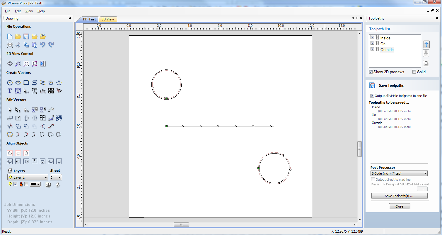
Guarde una trayectoria de herramienta con su postprocesador base y véala con su editor de texto favorito. A continuación se muestra un ejemplo del archivo de prueba publicado con el postprocesador "G-Code Arcs (pulgadas) (*.tap) el ejemplo siguiente se muestra utilizando el popular editor Bloc de notas++.
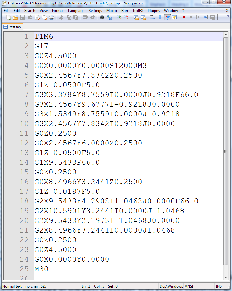
Para nuestro ejemplo, agregaremos una sección de cambio de herramienta a este postprocesador. En primer lugar, haga una copia segura del postprocesador que está personalizando. Si abre el postprocesador que está editando en un editor de texto, podrá ver las líneas de texto dentro del postprocesador que formateó la salida del archivo de prueba.
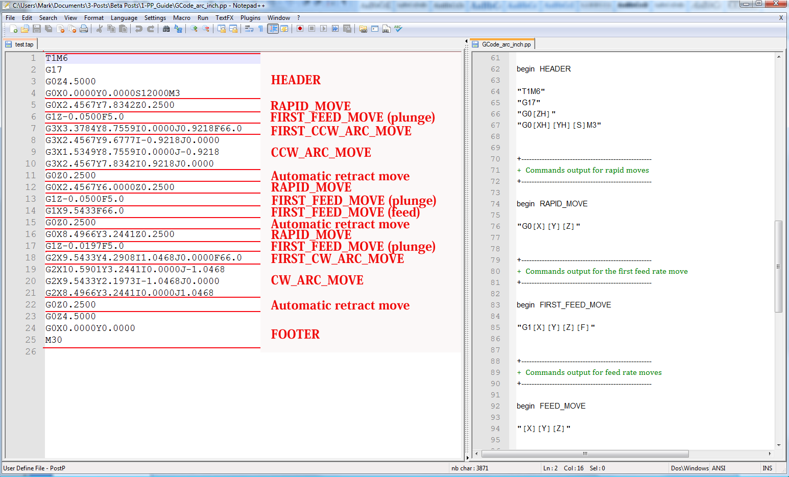
Se puede acceder a la carpeta PostP desde la aplicación, haciendo clic en "Archivo > Abrir carpeta de datos de la aplicación" en el menú principal de la aplicación.
Para agregar una sección de cambio de herramienta al postprocesador, deberá consultar la documentación para el control de la máquina herramienta (o software de control). En este ejemplo, asumiremos que las instrucciones que necesita agregar para realizar un cambio de herramienta para su máquina herramienta en particular son las siguientes:
- M05, Instrucción de apagar el husillo antes del cambio de herramienta.
- M0, Instrucción para devolver la herramienta existente al portaherramientas.
- M06TTool_Number n, Instrucción para seleccionar una nueva herramienta Tool_Number n
- G43HTool_Number n, Instrucción de control para utilizar el desplazamiento de longitud de herramienta para la herramienta n
- Sxxx M03, Ajusta la velocidad del husillo a xxx; Enciende el husillo (rotación en el sentido de las agujas del reloj).
Edita el postprocesador usando tu editor de texto favorito.
Si el sistema operativo del equipo está habilitado para Microsoft Vista y el Control de acceso de usuario está habilitado, copie o mueva el postprocesador que está editando desde la carpeta PostP a una carpeta debajo del área de usuario.
Lo primero que debe editar dentro del archivo es la sección Comentarios de historial; Para que tenga un registro de los cambios.
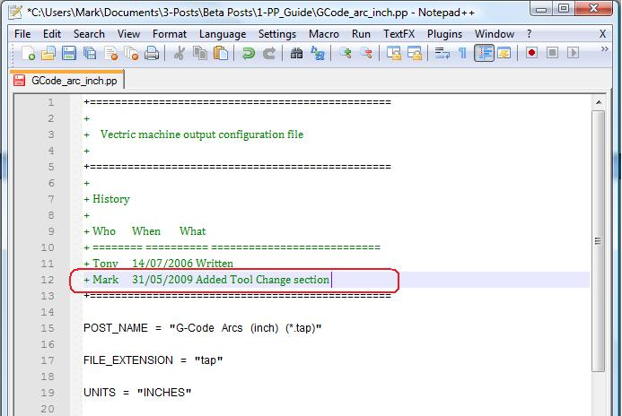
A continuación, edite POST_NAME para reflejar que este postprocesador genera comandos de cambio automático de herramientas (ATC), el nuevo post se mostrará como "G-Code ATC Arcs (inch)(*.tap)" en la lista de postprocesadores.
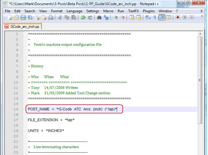
A continuación, agregue una sección de cambio de herramienta que incluirá las instrucciones. La ubicación de la nueva sección dentro del archivo no es importante, pero un buen lugar para insertarla es entre las secciones Header (encabezado) y Rapid Move (movimiento rápido).
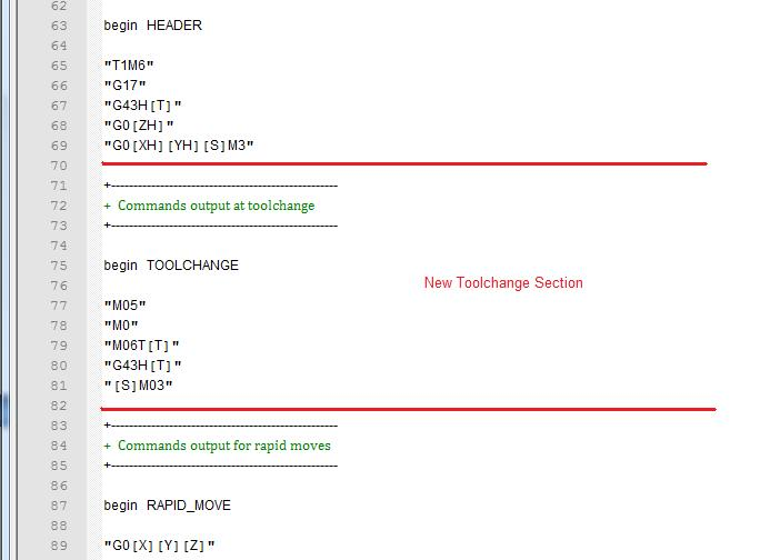
Agregue algunas líneas de comentario en la parte superior de la nueva sección, (comenzando por el carácter +) para describir la sección y hacer que el archivo en su conjunto sea más fácil de leer. A continuación, introduzca la línea "begin TOOLCHANGE" para indicar al postprocesador que se van a generar las siguientes instrucciones para cada cambio de herramienta (excepto la selección inicial de la herramienta, los comandos para estos están contenidos en la sección de encabezado).
El siguiente paso es introducir las instrucciones que necesite, entre comillas dobles. La "[T]" en la tercera y cuarta líneas de instrucción de nuestro ejemplo, se sustituirá por el número de herramienta cuando se procese el archivo; La "[S]" de la quinta línea se sustituirá por la velocidad del husillo de la herramienta.
Por último, tendrá que guardar los cambios en el archivo, ya que ha cambiado POST_NAME, guarde el archivo con un nuevo nombre, por ejemplo "GCODE_ATC_Arcs_inch.pp"
Si el sistema operativo del equipo es Microsoft Windows 7 o Microsoft Vista y el Control de acceso de usuarios está habilitado, copie el archivo que ha editado en la carpeta "PostP".
Para probar el nuevo postprocesador, si el software se está ejecutando, reinicie el software.
Si hay algún error de sintaxis con su postprocesador, se mostrará un error similar a la imagen siguiente cuando se inicie el software, el postprocesador que ha editado no aparecerá en la lista desplegable de archivos de configuración del postprocesador. Tendrá que corregir cualquier error y reiniciar el software.
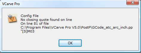
Si no se muestran errores cuando se inicia el software, abra el archivo de prueba y guarde una o varias de las rutas de herramientas de prueba.
Seleccione el postprocesador en la lista desplegable de la configuración del postprocesador y pulse el botón "Guardar trayectoria(s) de herramienta".
Echa un vistazo al archivo que acabas de guardar en un editor de texto.
Si el contenido del archivo se ve bien, prueba el archivo en el equipo.
Por favor, tome todas las precauciones necesarias al ejecutar la salida de un postprocesador modificado por primera vez.
Ejemplo: Cambiar la extensión de archivo
La extensión de archivo que es producida automáticamente por el postprocesador se puede cambiar dentro del cuadro de diálogo "Guardar como", al hacer clic en el botón "Guardar trayectoria(s) de herramienta".
Sin embargo, en lugar de cambiar la extensión de archivo cada vez. Es más conveniente cambiar permanentemente la extensión de archivo producida por el postprocesador.
Para hacer esto:
Haga una copia segura del postprocesador que desea editar.
Los archivos de configuración del postprocesador se encuentran en la carpeta "PostP" de la carpeta de instalación del producto y tienen ". PP" de extensión de archivo. Para Aspire versión 2, la ubicación predeterminada de la carpeta PostP es: "C:\Archivos de programa\Aspire V2.0\PostP". La ubicación de la carpeta PostP será diferente dependiendo del producto instalado y si el software se instaló en una ubicación personalizada durante la instalación.
Edita el postprocesador usando tu editor de texto favorito.
Si el sistema operativo del equipo está habilitado para Microsoft Windows 7 o Microsoft Vista y el Control de acceso de usuarios está habilitado, copie o mueva el postprocesador que está editando desde la carpeta PostP a una carpeta debajo del área de usuario.
Busque las dos líneas siguientes dentro del archivo de configuración del postprocesador que comienzan por:
POST_NAME =
FILE_EXTENSION =
y modifíquelos en consecuencia.
Por ejemplo, si desea cambiar la extensión de archivo producida por el postprocesador "G Code ATC (inch)(*.tap)" de ".tap" a ".nc". A continuación, edite las líneas:
POST_NAME = "G Code ATC (inch) (*.tap)"
FILE_EXTENSION = "tap"
para que se lean:
POST_NAME = "G Code ATC (inch) (*.nc)"
FILE_EXTENSION = "nc"
Guarde los cambios en el archivo. Si el sistema operativo del equipo es Microsoft Windows 7 o Microsoft Vista y el Control de acceso de usuarios está habilitado, copie el archivo que ha editado en la carpeta "PostP".
Para probar el nuevo postprocesador, si el software se está ejecutando, reinicie el software. Si hay algún error de sintaxis con su postprocesador, se mostrará un error similar a la imagen siguiente cuando se inicie el software, el postprocesador que ha editado no aparecerá en la lista desplegable de archivos de configuración del postprocesador. Tendrá que corregir cualquier error y reiniciar el software.
Si no se muestran errores cuando se inicia el software, abra el archivo de prueba y guarde una o varias de las rutas de herramientas de prueba.
Seleccione el postprocesador en la lista desplegable de la configuración del postprocesador y pulse el botón "Guardar trayectoria(s) de herramienta".
Echa un vistazo al archivo que acabas de guardar en un editor de texto.
Si el contenido del archivo se ve bien, pruebe el archivo en el equipo.
Por favor, tome todas las precauciones necesarias al ejecutar la salida de un postprocesador modificado por primera vez.
Consejos y trucos
- Siempre haga una copia segura del postprocesador que está editando, en caso de que necesite empezar de nuevo desde cero.
- Si utiliza un programa de procesador de textos, como Microsoft Word, para editar un postprocesador, asegúrese de que el archivo se guarda como texto sin formato. El archivo no debe contener información de formato.
- Si edita postprocesadores en un equipo que ejecuta Microsoft Windows 7 o Microsoft Vista, no edite los archivos directamente en la carpeta "Archivos de programa\Carpeta de producto\PostP". Edite siempre el archivo dentro de su área de usuario y copie el archivo editado en "Archivos de programa\carpeta de productos\PostP".
- Utilice comentarios cuando realice cambios, un comentario es un texto que sigue a un signo + o un caracter | . Los comentarios no serán actuados por el programa, pero pueden ayudar a documentar los cambios que ha realizado y hacer que esos cambios sean comprensibles en el futuro.
- Todas las líneas de instrucción deben estar contenidas entre comillas.
- Si es posible, utilice un editor de texto que haga uso de números de línea; Esto facilitará la depuración del postprocesador si hay algún error en el archivo. El programa comprobará los postprocesadores en la carpeta PostP cuando se inicie el programa. Si hay errores de sintaxis en el archivo, se mostrará un mensaje de error que muestra el número de línea del primer error encontrado.
- Una vez que haya editado correctamente un postprocesador, haga una copia segura del mismo. Si instala una versión posterior del producto Vectric que está utilizando, recuerde copiar el postprocesador modificado en la carpeta PostP de la nueva versión del software. Y seleccione su postprocesador modificado, la primera vez que guarde una trayectoria de herramienta, (el software recordará su selección para acciones posteriores).
- Si instala otra versión del software o actualiza la versión del software, recuerde copiar las copias seguras de los postprocesadores editados a la carpeta PostP de la nueva versión. Asegúrese de seleccionar el postprocesador correcto la primera vez que publique un archivo con la nueva versión del software.
- Para versiones posteriores del software, (V5.5 y superior). Se debe acceder a los postprocesadores desde la aplicación, haciendo clic en "Archivo > Abrir carpeta de datos de la aplicación\Carpeta PostP.
- Se puede crear una lista personalizada de postprocesadores copiando solo los postprocesadores necesarios en la carpeta "Archivo > Abrir Carpeta de datos de la aplicación\My_PostP. Si existe algún archivo con una extensión de archivo .pp en la carpeta "My_PostP", solo los postprocesadores que existen en la carpeta My_PostP se mostrarán en la lista desplegable de postprocesadores.