User Guide
- 2Dデザインと管理
- インターフェイス概要
- 2Dデザインと管理
- 3D Design and Management
- 3D Toolpath Files
- Rotary Machining and Wrapping
- Creating a Rotary Job
- Importing External Models in a Rotary Project
- Simple Rotary Modelling using 2D Toolpaths
- Modelling 3D Rotary Projects
- Advanced Modelling of 3D Rotary Projects
- ポストプロセッサ編集
2Dデザインと管理
2Dビューは、完成品のレイアウトのデザインと管理に使用されます。異なる要素を利用して、2Dのみのアイテム、または3Dビューでオブジェクトの2D表現であるアイテムの制御が可能です。ここでは、2Dビュー要素の一覧を簡単に説明しています。詳細は、マニュアルの関連するセクションを参照してください。
異なるタイプのオブジェクトを使用して、CNCでパーツの加工を行う際に必要な工具経路の作成が可能です。また、3Dモデルのベースや工具経路の境界形状の作成にも利用できる場合があります。2Dアイテムには異なるアプリケーションや利用法があるため、正しい管理が非常に重要です。そのため、Aspireは2Dデータを管理するためにレイヤ機能を提供しています。レイヤを使用して異なる2D要素を関連付け、より効果的に管理できるようにします。レイヤの詳細は、マニュアルの関連するセクションを参照してください。両面プロジェクトの作成時には、同一セッション内で「表面」と「裏面」を切り替えることができます。これにより、各面の作成と編集が可能で、[両面ビュー]オプションを使用して反対側のベクトルを表示することができます。両面セットアップの詳細は、マニュアルの関連するセクションを参照してください。
 ベクトル
ベクトル
ベクトルは線、円弧、カーブで、シンプルな直線から複雑な2Dデザインを構成するものまであります。ベクトルは工具形状がたどる形状や、2レールスイープなどの3Dモデリング機能と併用する2D形状のコントロールなど、Aspireで多用されます。ASPIREには多くのベクトル作成/編集ツールが含まれています。詳細は、マニュアルの関連するセクションを参照してください。
ソフトウェア内でのベクトルの作成に加え、Corel DrawやAutoCADなどのその他のデザインソフトウェアからのインポートも可能です。ASPIREでは*.dxf、*.eps、*.ai、*.pdf、*skp、*svgベクトルフォーマットのインポートがサポートされています。インポートが完了したら[ベクトル編集]ツールを使用し、ソフトウェア内でデータの編集や組み合わせが可能です。
ビットマップ
ビットマップは*.bmp、*.jpg、*.gif、*.tif、*.png、*.jpegのピクセルベースのイメージ(写真など)の標準のコンピューター用語です。これらのファイルタイプは非常に小さな正方形(ピクセル)に構成されるイメージで、スキャンされた写真、デジタル写真、インターネットから入手したイメージなどが相当します。
3Dモデルの作成を簡素化するために、Aspireでは「コンポーネント」と称される管理可能なピースにデザインを分割することができます。2Dビューでコンポーネントはグレースケール形状で表示され、選択、編集、移動、サイズ変更などが可能です。グレースケールを使用した作業方法は、マニュアルの関連するセクションを参照してください。ビットマップと同様に、選択したコンポーネントグレースケールで多くのベクトル編集ツールを利用することができます。
インターフェイス概要
- メインメニューバー(ドロップダウンメニュー):画面上部にあるこのバーには、ファイル、編集、モデル、工具経路、表示、ヘルプの各メニューが表示されます。ここから、機能別に分類されたソフトウェアのコマンドにアクセスすることができます。いずれかのメニューをクリックすると、利用可能なコマンドが記載されたドロップダウンリストが表示されます。
- デザインパネル:画面の左側に表示されます。デザインタブとタブ内のデザインを作成するためのアイコンへのアクセスが可能です。
- 工具経路タブ:画面の右側に表示されます。工具経路タブの上部には、工具経路の作成、編集、プレビューを行うための全アイコンが表示されます。タブの下部には作成済みの工具経路が表示されます。
- 2Dデザインウィンドウ:加工用デザインの表示、編集、選択を行うためのウィンドウです。デザインはインポートまたはソフトウェアで直接作成することができます。これは3Dビューでも同様で、F2キーとF3キーの使用、またはウィンドウ上部のタブをクリックして切り替えることができます。
- 3Dビュー:合成モデル、工具経路、工具経路プレビューが表示されます。
- インターフェイスレイアウトボタン(作図タブの2Dビューコントロールセクション):2Dビューと3Dビューを同時表示、またはデザインの後期工程で工具経路タブへフォーカスを切り替える場合に使用し、異なる既定のインターフェイスレイアウト間を切り替えます。
インターフェイスの管理
ツールタブは自動表示/非表示動作を採用しているため、使用していない場合は自動的に閉じられます。これにより、画面上の作業領域が最大になります。
ソフトウェアにはデザイン用と加工用の2つのデフォルトレイアウトが含まれており、自動的かつ容易に各ツールページの自動非表示の適切な動作を設定することができます。各ツールページのレイアウト切り替えボタンを使用して、プロジェクトのデザインステージから工具経路ステージにフォーカスが自然的に移動するようにインターフェイスを切り替えることができます。
自動非表示タブへのアクセス
ツールページが自動非表示(ピン付けされていない)の場合、画面のサイドにタブのみとして表示されます。詳細は、ツールページのピン付け/ピンを外すを参照してください。当該タブにマウスオーバーすると、一時的にページが表示されます。ページからツールを選択すると、再度自動的に非表示になります。
ツールページのピン付け/ピンを外す
各ツールページの自動非表示動作は、各ページのタイトル領域の右上にある画びょうアイコンを使用して制御可能です。
デザイン/工具経路のデフォルトレイアウト
Aspireには、通常のデザインワークフローと工具経路作成を補助するための2つのツールレイアウトページがあります。
すべてのタブに[レイアウト切り替え]ボタンがあります。作図とモデリングタブで当該ボタンを使用すると、工具経路タブをピン付けして作図とモデリングツールタブのピンを外し、工具経路タスクにインターフェイスのフォーカスが移動されます。工具作成タブでは、当該ボタンによってレイアウトが元に戻されます。つまり、工具経路ページのピンを外して作図とモデリングタブのピン付けを行います。これらの2つのタブは、F11キーとF12キーを使用して切り替え可能です。
2Dデザインと管理
2Dビューは、完成品のレイアウトのデザインと管理に使用されます。異なる要素を利用して、2Dのみのアイテム、または3Dビューでオブジェクトの2D表現であるアイテムの制御が可能です。ここでは、2Dビュー要素の一覧を簡単に説明しています。詳細は、マニュアルの関連するセクションを参照してください。
異なるタイプのオブジェクトを使用して、CNCでパーツの加工を行う際に必要な工具経路の作成が可能です。また、3Dモデルのベースや工具経路の境界形状の作成にも利用できる場合があります。2Dアイテムには異なるアプリケーションや利用法があるため、正しい管理が非常に重要です。そのため、Aspireは2Dデータを管理するためにレイヤ機能を提供しています。レイヤを使用して異なる2D要素を関連付け、より効果的に管理できるようにします。レイヤの詳細は、マニュアルの関連するセクションを参照してください。両面プロジェクトの作成時には、同一セッション内で「表面」と「裏面」を切り替えることができます。これにより、各面の作成と編集が可能で、[両面ビュー]オプションを使用して反対側のベクトルを表示することができます。両面セットアップの詳細は、マニュアルの関連するセクションを参照してください。
ベクトル
ベクトルは線、円弧、カーブで、シンプルな直線から複雑な2Dデザインを構成するものまであります。ベクトルは工具形状がたどる形状や、2レールスイープなどの3Dモデリング機能と併用する2D形状のコントロールなど、Aspireで多用されます。ASPIREには多くのベクトル作成/編集ツールが含まれています。詳細は、マニュアルの関連するセクションを参照してください。
ソフトウェア内でのベクトルの作成に加え、Corel DrawやAutoCADなどのその他のデザインソフトウェアからのインポートも可能です。ASPIREでは*.dxf、*.eps、*.ai、*.pdf、*skp、*svgベクトルフォーマットのインポートがサポートされています。インポートが完了したら[ベクトル編集]ツールを使用し、ソフトウェア内でデータの編集や組み合わせが可能です。
ビットマップ
ビットマップは*.bmp、*.jpg、*.gif、*.tif、*.png、*.jpegのピクセルベースのイメージ(写真など)の標準のコンピューター用語です。これらのファイルタイプは非常に小さな正方形(ピクセル)に構成されるイメージで、スキャンされた写真、デジタル写真、インターネットから入手したイメージなどが相当します。
3Dモデルの作成を簡素化するために、Aspireでは「コンポーネント」と称される管理可能なピースにデザインを分割することができます。2Dビューでコンポーネントはグレースケール形状で表示され、選択、編集、移動、サイズ変更などが可能です。グレースケールを使用した作業方法は、マニュアルの関連するセクションを参照してください。ビットマップと同様に、選択したコンポーネントグレースケールで多くのベクトル編集ツールを利用することができます。
3D Design and Management
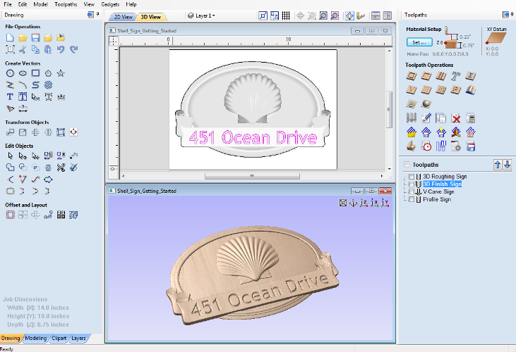
As well as creating toolpaths directly from 2D drawings, Aspire can produce extremely flexible 3D toolpaths. These toolpaths are created from 3D design elements called 3D Components that can be generated from models created in external 3D design packages, imported as 3D clipart or built entirely from within Aspire using 2D artwork as a source.
The 3D View
The 3D View can show you the current Composite Model (which is built from all of the currently visible 3D Components and Levels), the Toolpath Preview (a highly accurate 3D simulation of the resulting physical object that will result from your toolpaths called the Preview Material Block). Which of these is currently displayed will depend on whether or not you have a part which has 3D Components and Toolpaths or are just working on something that only includes 2D Data.
Whenever you have the Preview Toolpaths form open on the Toolpaths tab, the 3D View displays the Preview Material Block instead of the Composite Model. When this is closed if you are working on a part that only includes 2D data and 2D or 2.5D toolpaths it will continue to display the Preview Material Block. If your part contains any visible 3D Components then as soon as the Preview Toolpaths form is closed it will revert to showing the Composite Model in the 3D View and hide the simulation. In addition to these items, you can see line drawings of any calculated toolpaths in the 3D View. The visibility of these calculated toolpaths can be controlled from the Toolpath List on the Toolpaths tab using the check-boxes next to the toolpaths name. If working in a 2 Sided environment you can view both sides of a project in the 3D View using the Multi Sided View option.
The Composite Model
Aspire has been designed to work in a way which enables the user to easily create even very complex projects. In any situation, the best approach to producing something complicated is to break it down into smaller pieces until a level of simplicity is reached that can be understood and managed. In Aspire this is achieved by letting the user work with pieces of the design which are combined to make the finished part. In the terminology of the software these pieces are called Components. To help organize the Components they are assigned to Levels. Step by step, Components and Levels can be created and modified until you have all the elements you need. In the images below you can see an example of how this might work. On the left you can see the separate component for a model of a bunch of grapes and on the right you can see these positioned to make the complete part - we call this resulting combination the Composite Model.
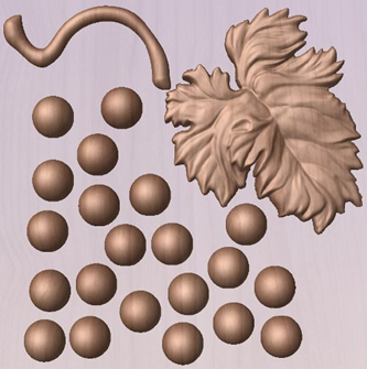
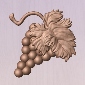
There is no limit to how simple or complex a Component or the Components on a Level can be (this is the user's choice). In the example shown, you can see that a model of a whole bunch of grapes may be made up of smaller individual components but they could also be combined to exist as one single Component (the assembled bunch of grapes) that could then be used to lay-out a more complex part with multiple bunches of grapes. They could also be organized so all the grapes were on one Level and leaf and stem on another to provide a different way of managing and manipulating the shapes. Each user will find a level of using Components and Levels they are comfortable with which may be dependent on the particular job or level of proficiency with the modeling tools.
3D Components and Levels
In Aspire, the aim is to end up with a set of Components and Levels that when combined together will make the finished 3D part. One way to think of this is like building a 3D collage or assembly. As the design evolves, new Levels or shapes may need to be created or existing ones changed. The parts of the collage are managed with the Component Tree which will be covered in more detail later.
Creating and Editing Components
An existing Component can be copied, scaled and have other edits carried out on it as an object. The user can also change the way it relates to the other Components, for instance whether it sits on top or blends into an overlapping area of another Component. The shape, location and relation of these pieces determine the look of the final part. As the job progresses, the user will need to create brand new Components or edit existing ones by adding new shapes, combining them with others or sculpting them.
Components can be created and edited by:
- Use a modelling tool to create shapes from 2D vectors.
- Import a pre-created 3D model - either a model previously created in Aspire or from another source such as a clipart library or a different modelling package.
- Create a 'texture' Component from a bitmap image.
- Use the Split Components Tool to break an existing Component into multiple pieces.
All of these methods are covered in detail throughout the training material.
Dynamic Properties
As well as having its underlying 3D shape, each component also has a number of dynamic properties that can be freely modified without permanently changing its true shape. These include scaling of the Component's height, the ability to tilt it, or to apply a graduated fade across it.
These dynamic properties can always be reset or altered at any time during your modeling process, which makes them a particularly useful way of 'tweaking 'your components as you combine them together to form your final composite model.
Combine Modes
The Combine Mode is a very important concept when working with 3D shapes within Aspire. The options for combine mode are presented when creating new shapes and also when deciding how Components and Levels will interact in the Component List. Rather than cover this in every section where it is applicable, it is worth summarizing the options here so the general concept can be understood.
When you have more than one 3D shape, such as the Component pieces of the design or where you have an existing shape and are creating a new one, then you need to have a way to tell the software how the additional entities will interact with the first. This can be an abstract concept for users who are new to 3D but it is an important one to grasp as early as possible. In Aspire this is controlled by a choice called the Combine Mode.
There are four options for this: Add, Subtract, Merge High, Merge Low.
As modeling is an artistic and creative process, there is no general rule to describe when to use each one. As a guide though you can assume that if the second shape's area is completely within the originals one then you will probably be adding or subtracting and if the shapes only partly overlap that you will probably use Merge or, very occasionally, Low.
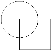
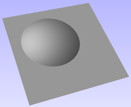
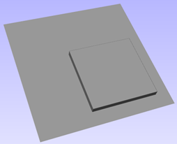
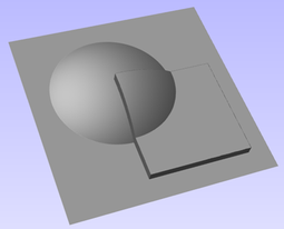
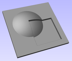
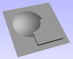
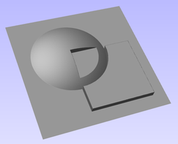
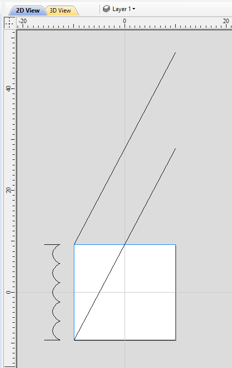
The four options and their specific effects are described on the following pages. To illustrate the different effects a combination of an overlapping beveled square and a dome will be used. You can see in the image top right how these are arranged in the 2D View and how they overlap. Then you can see each individual shape in the images below middle and right. These shapes will be used to demonstrate the different Combine Modes. In every case the Dome will be considered the primary shape and the square is the secondary shape which is being combined with the first. In addition to the dome/square example some images of 'real world' parts will also be included to help to understand how these can be used on actual projects.
As well as working on individual shapes, the Combine Modes are also assigned to Levels. These will govern how the combination of all the individual components on one Level interacts with the result of all the Components on the Level below it in the Component Tree
Note:
There is a 5th Combine Mode available from the right mouse click menu after a component has been created called Multiply. This combine mode has specialist applications which are dealt with in the appropriate tutorial videos. This option will literally multiply the heights of the Component or Levels being combined to create the new Composite 3D shape.
Add
When Add is selected, it takes the first shape and then just adds the height of the second shape directly on top of the first. Any areas which overlap will create a shape which is exactly the height of each shape at that point added together (see below)
Typically the add option is mainly used when the shape being added sits completely within the original shape, this ensures that the uneven transition where the parts only partly overlap (as shown in the example) do not occur.
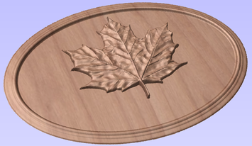
The example above shows the Maple Leaf and border extrusion Components being Added to the dome Component in the sign example from the Introduction to Modeling document.
Subtract
When Subtract is selected it takes the first shape and then removes the height of the second shape from the first. Any areas which overlap will be a combination of the original height/shape less the second shape. Areas where the shape goes into the background will become negative regions. You can see how this looks using the dome and square in the image below:
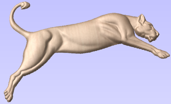
Typically subtract, like the add option, is mainly used when the shape being removed sits completely within the original shape, this ensures that the uneven transition where the parts only partly overlap (as shown in the example) do not occur.
The image shown above has some 'creases' to help define the muscles of the lioness. The shapes to create these recesses were created by using the Subtract option with the Create Shape tool on the vectors representing those recessed areas.
Merge
When the Merge option is selected any areas of the shapes which do not overlap remain the same. The areas that overlap will blend into each other so that the highest areas of each are left visible. This results in the look of one shape merging into the other and is in effect a Boolean union operation. You can see how this looks using the dome and square in the image below:
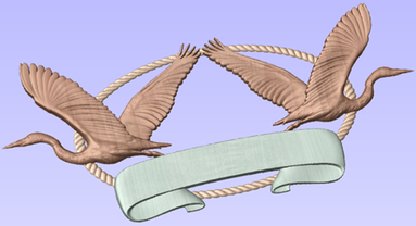
Typically the merge option is used when the shape being combined partly overlaps the original shape. This enables a reasonable transition to be made between them.
The image above shows 2 Herons, a rope border and banner Components. Each of these overlaps with the others and so they are set to Merge in this areas. Whatever is the higher of the two merged areas is what is prominent. In this case the rope is lower than everything and the Banner is higher than the Herons so the desired effect can be achieved.
Low
The Low option is only available when combining Components (not in the modeling tools). When this mode is selected, any areas which do not overlap are left as they were in the original two shapes. Any areas which overlap will create a new shape which is the lowest points taken from each shape, this is in effect a Boolean intersection operation. You can see how this looks using the dome and square in the image below:
The Low option is used for recessing a shape into a raised shape. An example of this is shown in the image above.
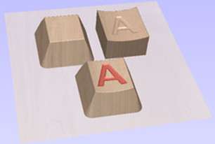
The example shown on the right above uses the Low option to combine the flat topped 'button' component on the left with the curved top face component with the letter 'A' on the right. Combining both components with the merge low option gives the keyboard button with the curved top you see in the bottom row.
Level Mirror Modes
Right-clicking Levels in the component tree will open a pop-up menu offering commands and operations related to the clicked level and Mirror Modes can be set in this way. If a mirror mode is set on a Level, all the components it contains will be continually mirrored dynamically as they are moved, transformed or edited. The mirroring is non-destructive, that is it can be turned off or on at any time and does not alter the underlying components in any permanent way. Working inside a Mirror modes Level is a simple way of achieving a complicated symmetrical pattern by editing only one half (or quarter, see below) of the design.
The available Mirror Modes are broadly divided into two groups. The first group apply one plane of symmetry:
- Left to Right
- Right to Left
- Top to Bottom
- Bottom to Top

These modes allow you to work in one half of your job and the other half will be automatically and dynamically generated for you. For example, in Left to Right mode you would place your components in the left half of your job and a mirrored equivalent of each would be created in the other half of the job. This 'reflection' is updated dynamically as you work.
The other group offer two planes of symmetry (horizontal and vertical):
- Top Left Quadrant
- Top Right Quadrant
- Bottom Left Quadrant
- Bottom Right Quadrant
When using these modes your components should all be in the quadrant (quarter) of the job. Mirrored reflections horizontally and vertically will be created in the other quadrants of the job for you.
Multi Sided View

When working in a 2 Sided environment you can create components independently per side or using the Right click option you can copy or move a component to the opposite side. Selecting the option to work in 'Multi Sided View' allows you to view components you may have on the Top and Bottom side in the 3D View. In the Toolpath Preview form of a project that contains toolpaths for the Top and Bottom Sides the multi sided view presents the simulation of the toolpath preview on both sides also, if the multi sided view is not selected you can use the 'Preview all Sides' option in the Toolpath Preview form to display the Top and Bottom Toolpaths in the 3D view. 2 Sided Setup will be described in detail later in the relevant section of this manual.
3D Toolpath Files
Files from Vectric's Cut3D, PhotoVCarve and Design and Make Machinist that include 3D toolpaths can be imported into Aspire using the main menu command: File ► Import ► PhotoVCarve, Machinist or Cut3D Toolpaths.
The 3D file must first be scaled to the required size before toolpaths are calculated, and then the complete file saved ready for importing into Aspire. These files can only be moved and positioned inside Aspire but cannot be scaled.
A Grayscale thumbnail of the 3D job is drawn in the 2D View with the X0 Y0 origin at the position it was set in Cut3D, PhotoVCarve or Design and Make Machinist. The associated toolpath(s) are also drawn in the 3D window and the names appear in the Toolpath list.
Positioning
To move the 3D design toolpaths open the 2D Window, click the Left mouse Twice on grayscale image (turns light Blue to indicate it's selected), then drag to the required position, or use the Move or Alignment tools for accurate positioning.
The toolpath(s) are automatically moved in the 3D window to the same XY position as the image.
Toolpaths for the example above have been calculated with the X0 Y0 in the middle of the 3D design. When imported into Cut2D the data is automatically positioned using the same coordinates, which places three quarters of the design off the job. In the second image the grayscale image has been moved to the middle of the job.
The 2D mirror and rotate drawing tools can also be used to edit the 3D data set.
3D toolpaths can also be copied using the Duplicate Toolpath command on the Toolpaths Tab making it very easy to use multiple elements from a single design on a job. The thumbnail preview is also copied for each toolpath, making it very easy to position additional copies of a 3D toolpath.
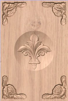
For example, a single design can be copied and mirrored to create Left and Right versions of a 3D design or to place multiple copies of a decorative design in the corners of a cabinet door panel as shown below.
Toolpaths for the 3D elements can be previewed along with the conventional Profile, Pocketing and Drilling toolpaths, and everything will be saved ready for machining.
A good example of where this functionality might be used in conjunction with PhotoVCarve is for making personalized picture frames that include the PhotoVCarve grooves plus descriptive engraved text and a decorative Profiled or Beveled border. As shown below:


Options
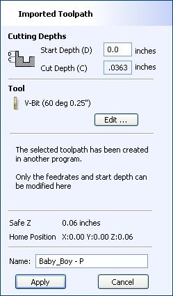
Imported toolpaths can also be edited to position them inside the material or to change the cutting parameters - speeds and feed rates can be changed.
Design and Make Machinist
When using a Design and Make Machinist file that includes multiple toolpaths, you must remember to edit the Start Depth for all of the imported 3D toolpaths.
Click the Edit toolpath icon or Double click on the toolpath name to open the edit form.
For example, after machining a half-inch deep pocket a PhotoVCarve design can then be edited to have a Start Depth = 0.5 inches and this will carve the photograph onto the base of the pocket surface.
Rotary Machining and Wrapping
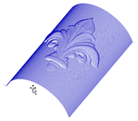
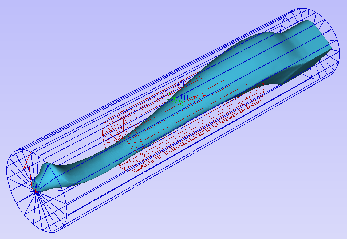
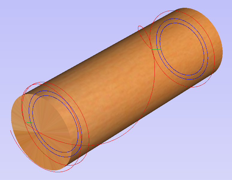
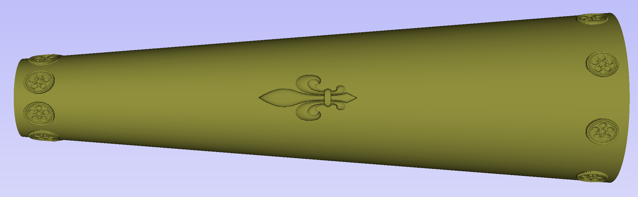
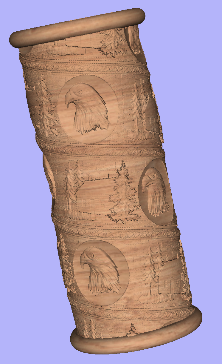
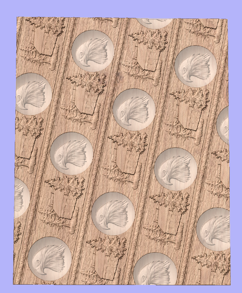
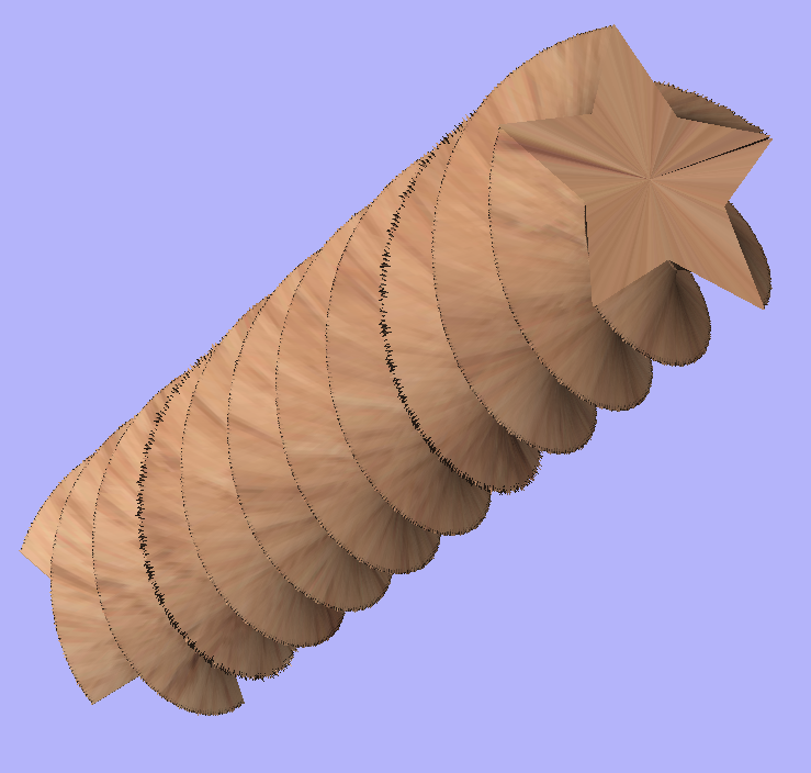
Aspire can 'wrap' flat toolpaths around a cylinder to provide output to CNC machines which are configured with a rotary axis / indexer. The image below shows a flat toolpath wrapped around part of a cylinder.
Note
It is important to note that wrapping works in conjunction with specially configured post-processors which take the XYZ 'flat' toolpaths and wrap them around a rotary axis, replacing either the X or Y moves with angular moves.
The toolpaths can be visualized wrapped within the program when the Auto Wrapping mode is on.
Aspire can also visualize a wrapped model within the program by drawing the shaded composite model wrapped.
Aspire also has the ability to draw the toolpath simulation wrapped. Although this is very useful for getting a feel for how the finished product will look, it is important to realize that the wrapped simulation may not be a 100% accurate representation of how the finished product will look. An example of potential difference would be if you drilled holes in your rotary job. In the actual work piece these will obviously just be round holes, in the wrapped simulation these may appear as distorted ovals due to the 'stretching' process which takes place when we wrap the flat simulation model for display.
Note
If your rotary axis is aligned along your Y axis you would choose the Orientation Along Y Axis option during job setup. All the examples in this document will assume that the rotary axis is aligned along X.
It is important to realize that there are a huge number of possible combinations of machine controller and axis orientations for rotary axis / indexers. This means it is impractical for Vectric to supply a pre-configured post-processor for every possible combination as standard. We include some wrapping post-processors in the software that can be configured when you setup your Machine Configuration.
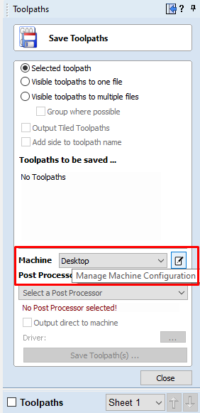
If you need to select a new post, you can do so by accessing the Save Toolpaths menu. To do so, click the 'Manage machine configuration' button as seen in the image below:
This will now open a menu where you can press the button under 'Associated Post-Processors' to access all of the available post-processors within the software and choose the appropriate wrapped post-processor for your machine configuration.
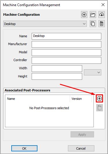
You can also right click the post in this menu and select 'view' to view the contents of the post, should you need to edit it later.
Examining these posts may be helpful if you need to configure a post of your own. If Vectric have not supplied a standard a post for your machine configuration please refer to the Post Processor Editing Guide accessible from the Help menu of the program for information on how to configure a post-processor and also look at the standard rotary posts Vectric supply.
You should also look at the Vectric forum to see if anyone else has already configured a post for your configuration or one similar. If, after looking at these resources you are still unsure of what needs to be done for your machine, please feel free to contact support@vectric.com for help. However, please note that we cannot guarantee to write a custom rotary post-processor for every individual requirement.
Creating a Rotary Job
Z Origin
You have the choice of specifying if the tool is being zeroed on the center of the cylinder or the surface. When you are rounding a blank, you cannot set the Z on the surface of the cylinder, as the surface it is referring to is the surface of the finished blank. We would strongly recommend for consistency and accuracy that you always choose 'Center of Cylinder' when outputting wrapped toolpaths as this should always remain constant irrespective of irregularities in the diameter of the piece you are machining or errors in getting your blank centered in your chuck.
Tip:
A useful tip for doing this is to accurately measure the distance between the center of your chuck and a convenient point such as the top of the chuck or part of your rotary axis mounting bracket. Write down this z-offset somewhere, and zero future tools at this point and enter your z-offset to get the position of the rotary axis center. Another reason for choosing 'Center of Cylinder' is that some controls will be able to work out the correct rotation speed for the rotary axis based on the distance from the center of rotation. If the Z value is relative to the surface, the control would need to know the diameter or radius of the cylinder at Z zero.
XY Origin
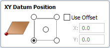
XY Drawing Origin - Here you can specify where the XY zero origin will be placed on your job. These options correspond to the same fields on the normal 'Job Setup' form within the program. Most people would use the default Bottom Left Corner, but for some jobs you may prefer to have the XY origin in the Center.
- In a job with horizontal orientation (Along X Axis), the X offset will correspond to the length of the cylinder, and the Y offset will be a point along its circumference.
- In a job with vertical orientation (Along Y Axis), it's the opposite. The Y offset will correspond to the length of the cylinder, and the X offset will be a point along its circumference.
Orientation
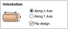
Cylinder Orientation Along - This section is used to tell the program how you have your rotary axis aligned on your machine. If you've already made your design, but just want to change the job for a different machine, then you could flip your design with the material so that all the vectors and components stay the same relative to the job.
Z Origin On - This section determines whether the Z Origin is set to the surface of the material or the base (center of cylinder). These settings can be over-ridden when the toolpath is actually saved, but we would strongly recommend the 'Cylinder Axis' is selected for rotary machining. The reasons for this are detailed in the note below.
Vector Layout
As well as creating a job at a suitable size for wrapping toolpaths, when creating the job, it will create a number of vectors which can be very useful when creating your wrapped job.
The vectors are created on their own individual layers and by default these layers are switched off to avoid cluttering up your work area. To switch on the layers, display the 'Layer Control' dialog (Ctrl+ L is the shortcut to show / hide this). To show / hide the layer simply click on the check box next to the layer name.
2Rail Sweep Rails - This layer contains two straight line vectors which can be used to sweep a profile along if you are creating a shaped column.
Bounding Box - This layer contains a rectangular vector covering the entire job area. This vector is useful if you are going to machine the complete surface of the cylinder.
Choosing stock material
When setting-up rotary project, software assumes a perfect cylinder with an exact diameter. In practice the stock material may be uneven, or only blank with square profile may be available. In those cases blank needs to be machined into cylinder of desired size, before running toolpaths associated with the actual design.
Another consideration is length of the stock material. Typically, part of the blank will be placed within the chuck. It is also important that during machining, the cutting tool is always in safe distance from both chuck and tailstock. For those reasons, the blank has to be longer than the actual design. When setting-up the machine for cutting, one has to pay extra attention to ensure that origin is set accordingly to avoid the tool running into chuck or tailstock!
If the design was created without those considerations in mind, the blank size can always be adjusted in the Job Setup form.
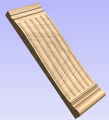
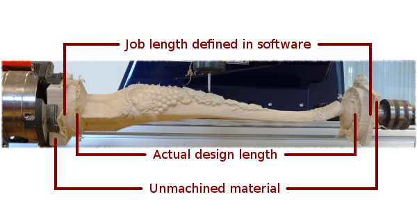
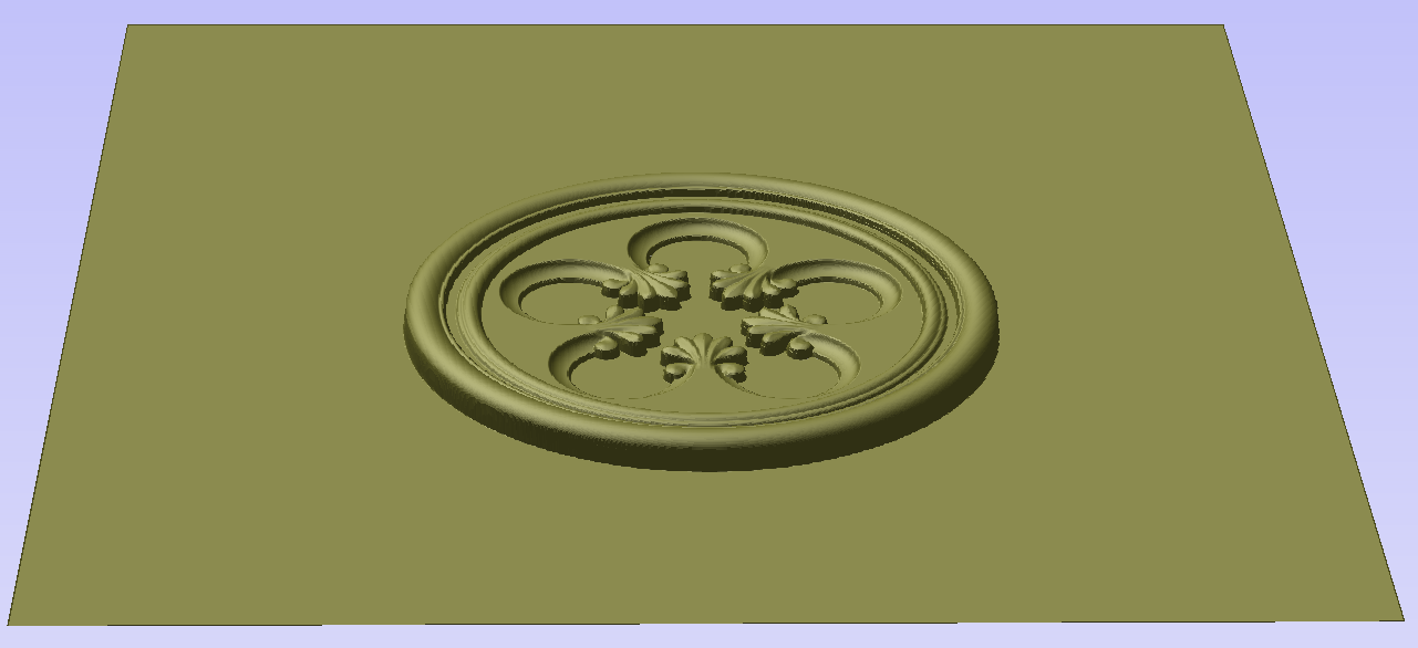
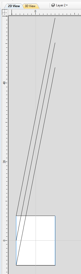
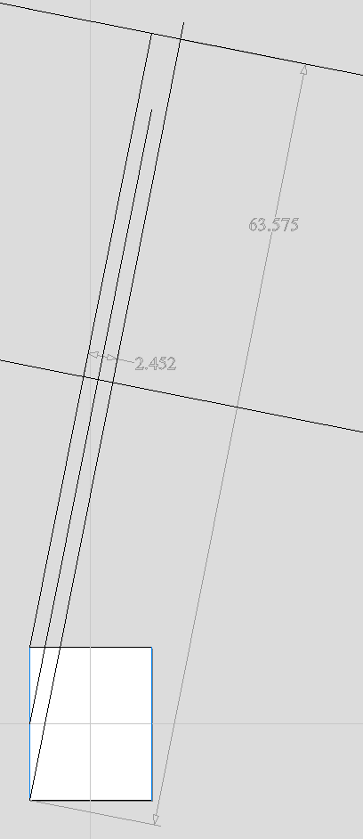
The picture below presents an example of a rotary project layout. As explained above, the actual blank is longer than job defined in Aspire to allow for the chuck and sufficient gaps. The actual design is shorter than job defined in Aspire, to leave some space for tabs, that can be machined with the profile toolpath prior to removing the finished part from the chuck.
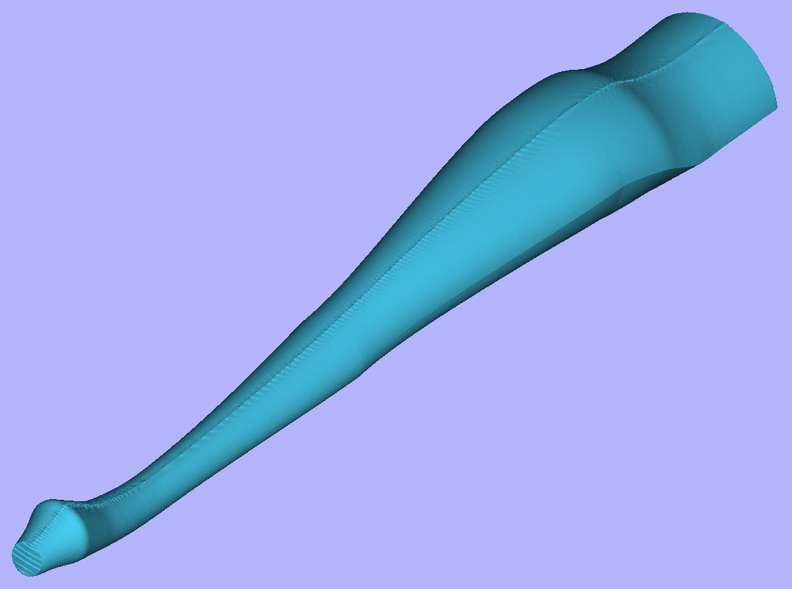
When machining 3D shapes with varying thicknesses like on the example shown below, it is a good idea to place the thicker end of the model on the side closest to the driving motor. This way torsional twisting will mostly affect the stronger end of the machined part and help to avoid bending or breaking of the part during machining.
Importing External Models in a Rotary Project
Importing Full-3D models
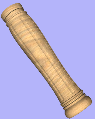
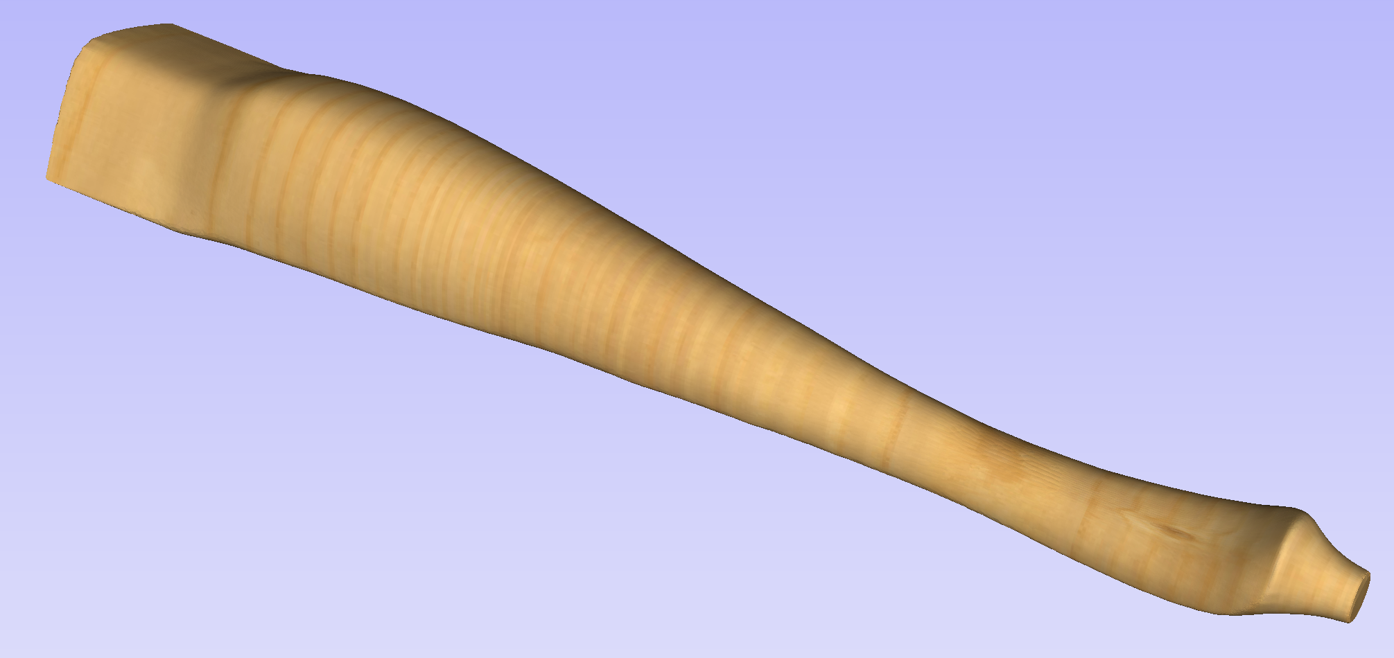
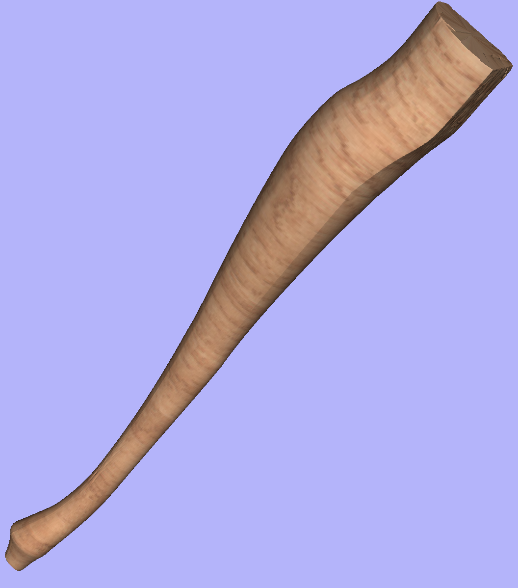
This section will present the process of importing the Full-3D STL model into rotary project, using a table leg as an example.
Overview
There are two basic use cases when importing an external model into the rotary job. The first case involves bringing a model designed for this particular job in another software. Thus the dimensions of the imported piece may already be correct and it can be desired to use them for the size of project. The second use case is when importing a stock model that would have to be scaled to fit on particular machine.
Aspire uses following workflow that covers both of those cases:
- Setting-up rotary project
- Choosing file for import
- Orientating the model in material block
- Scaling the model
- Finishing the import
Setting up a rotary project
Create a new job using the Job Setup form. It is important to set the job type as rotary to ensure a proper import tool is used in the next step.
If the dimensions of the project are already known, they could be specified directly.
If it is desired to fit the model to a given machine or stock available, set both the diameter and length to maximum. During import the model will be scaled to those limits.
If it is desired to use the imported model size, any size can be specified at this time. During the model import the project can be automatically resized to match the model dimensions.
In this example it was desired to fit the model into a specific stock size with a Diameter of 4 inches and a Length of 12 inches. XY origin was set to centre.
Importing the file and orientating it
To start the importing process, use Import a Component or 3D Model tool from the Modelling tab
Make sure that the Imported model type is set to Full 3D model .
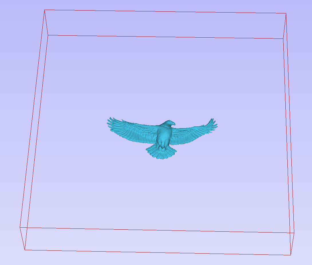
The first step is to position the imported model within the material. This step is necessary as this information is not present in the imported file. When the model was opened, the import tool chose the initial orientation, as can be seen below.
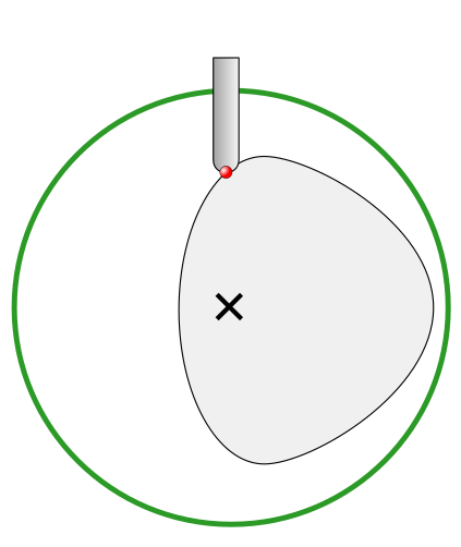
To help with orientating the model, the software displays a blue bounding cylinder. This cylinder has the rotation axis aligned with that defined for the material block and thus can be used as a reference. Its size is just big enough to contain the imported model at the current orientation. When the model orientation is changed, this blue cylinder will shrink or grow so it always contains the model. At this stage its exact dimensions are not important, as we are only interested in positioning the model correctly.
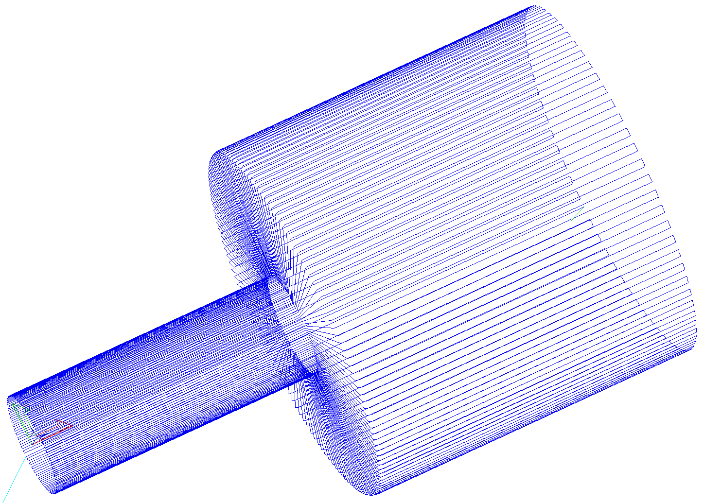
The software also highlights the rotation axis in red. This is particularly important when importing bended models. It is currently not possible to represent areas of model that are entirely below or above the rotation axis. This is the case in the example shown here. If the model was imported as is, the distortion would be created as can be seen below. Therefore it is important to position the model in a way such that the rotation axis is contained within the model.
The last guiding element displayed by the software is the red half arrow on the side of the cylinder. This arrow is indicating the position that corresponds to the center of the wrapped dimension in the 2D view. In this example the model is orientated in such a way, that front of the leg would be placed on side of the 2D view, rather than centre. Thus it is better to rotate model so this arrow points to the front of the imported model.
The import tool provides a few ways of adjusting the model orientation. The most basic one is the Initial Orientation. This can be used to roughly align the model with the rotation axis. This can also be combined with the Rotation about Z Axis.In this example the tool chose Left with no rotation. In order to align the front of the leg with the red arrow, one could use the Front and -90 as the Rotation about Z Axis.
Once the initial orientation is decided, further adjustments can be made using the Interactive Rotation. The default option - XYZ View - disables the interactive rotation. That means that the 3D view can be twiddled with a mouse. Selecting other options enables the rotation around the specified axis.
In this example, instead of changing the initial orientation to align the front of the leg with the red arrow, one could select X Model option and rotate the piece manually. When selecting single axis rotation, the 3D view will be adjusted to show that axis pointing towards the screen. If any mistake is made, it is possible to undo rotation using Ctrl+ Z
Notice that whenever the part is rotated, it is always centered in the cylinder. In this example it is not desired, since we need the rotation axis to be contained within the model. In order to move the model in relation to the rotation axis, one can use the Rotation Axis Movement
Similarly to the previously described tool, when Rotation Axis Movement is set to Off, the 3D view can be panned
Correctly positioning the model for importing may require a combination of the Rotation Axis Movement and the Interactive Rotation to achieve desired results with models that bend. It is important to make sure that rotation axis is hidden in order to avoid distortion. However it is also desirable to have the rotation axis being in the center of each segment of the piece to ensure tool has angle close to the optimal during machining. Usually it is also useful to rotate the model in view around the axis after the adjustment, as this allows us to inspect the model from each side without the need to disable the Interactive Rotation before changing the viewing angle.
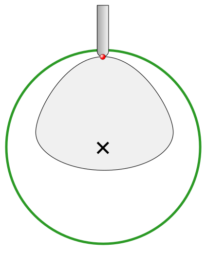
It is important to understand that Aspire does not support 4-axis machining. That means that while the machined piece can be rotated and tool moves along the rotation axis and in the Z direction, it is not possible to move the tool in the wrapped dimension and thus the tool is always above the rotation axis and cannot be moved to the side.
This limitation is shown below. The first picture presents correct machining of the point. If the tool moves to another location though, the angle will be incorrect and even worse, the tool side will be touching the stock.
Scaling imported model
Once model has been positioned as desired, its size can be taken into account.
By default the tool will assume that imported model is using the same units as the project. If that is not the case, model units can be switched. In this example project was set-up in inches, while imported model was designed in mm. After switching model becomes considerably smaller and a red cylinder, representing current material block is shown, as can be seen below.
At this point it is possible to specify the model size, in terms of diameter and length. This can be done manually by typing desired dimensions, or by fitting to material. If Lock ratio option is selected, the ratio between diameter and length is kept. One can also tick Resize material block option. If it is selected, the material block will be scaled to match current size of the model, after OK is clicked.
If it is desired to use model size as material block size, one can just make sure units are correct, then tick Resize material block option and press OK.
If it is desired for the model to fit material, one could click Scale model to fit material and tick Resize material block.
In this example model was fitted to material. Since in this case length of the piece is limiting factor and lock ratio is maintained, this results in model having considerably smaller diameter than material block. Hence Resize material block option was ticked.
Finishing import
After pressing OK the model will be imported as a component. It is possible to modify it as any other component or add pieces of decorative clipart onto its surface if desired.
It is important to keep in mind the distortion caused by the wrapping process. That means that wrapped toolpaths will match flat toolpaths only at the surface of the blank. The closer to the rotation axis (i.e. deeper) the toolpath is, the more it will be 'compressed'. This fact have a profound implication for 3D toolpaths. Consider the example shown below.
As can be seen if there is substantial difference in diameter in different parts of model, generating one 3D toolpath for whole model will result in wrapped toolpath being overly compressed. Thus it is usually better to create boundaries of regions with significantly different diameter and generate separate toolpaths using correct settings for each diameter.
Importing Flat Models
This section will present a process of importing Flat STL model into rotary project. Flat models are similar to decorative clipart pieces provided with Aspire and are supposed to be placed on the surface of modelled shape.
To start the importing process, use Import a Component or 3D Model tool from the Modelling tab
Make sure that Imported model type is set to Flat model
Again the first step is to select proper orientation of model. The tool will chose initial orientation and display model in the red material box. This box corresponds to the 'unwrapped' material block and its thickness is equal to half of the specified diameter of the blank.
If model is not oriented correctly, that is, does not lie flat on the bottom of the material box, as can be seen above, orientation have to be adjusted. To do that one can change Initial Orientation option and/or Rotation about Z Axis.
If imported model is not aligned with any of the axes, it may be necessary to use Interactive Rotation.The default option - XYZ View - disables interactive rotation. That means that 3D view can be twiddled with a mouse. Selecting other options enables rotation around specified axis.
Each rotation can be undone by pressing Ctrl+ Z.
Once model is properly orientated, units conversion can be performed. By default the tool will assume that imported model is using the same units as the project. If that is not the case, model units can be switched.
There is also model scaling option included. When Lock ratio option is selected, the ratio between X, Y and Z lengths are kept. Note that once model is imported, it will be added to project as a component. Hence correct placement, rotation and sizing can be performed later, after model is imported.
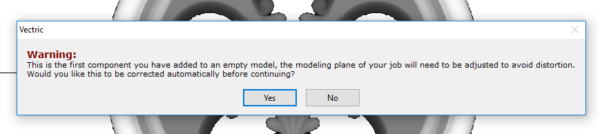
If the project does not contain any models yet, following message will be displayed:
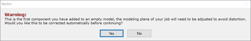
Typically you could simply click Yes.The more detailed explanation about modelling plane adjustment has been provided in Modelling 3D rotary projects
Simple Rotary Modelling using 2D Toolpaths
Creating vectors for a basic column
This section will show how to create a simple column, using the profile and fluting toolpaths.
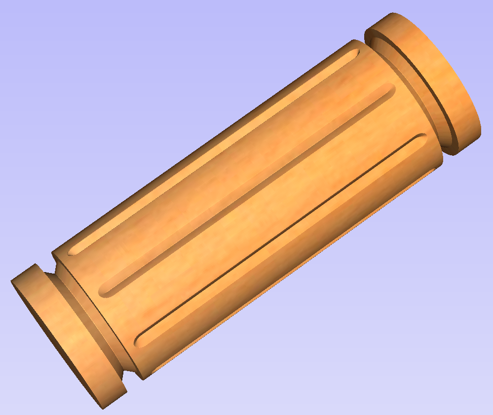
Start by creating a new rotary job. Please note that settings shown here are only an example and should be adapted to match your machine setup and available material.
In this example the blank will rotate around X axis. We will refer to it as the rotation axis. The axis that will be wrapped is the Y axis. We will refer to it as the wrapped axis. That means that the top and bottom boundaries of the 2D workspace will actually coincide. We will refer to them as the wrapped boundaries.
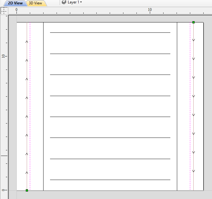
First, create the cove vectors using Draw Line/Polyline tool. Those will run along the wrapped axis at both ends of the design. Snapping may be useful to ensure that the created line starts and ends at the wrapped boundaries.
In this example the coves were placed 1 inch from the job boundaries, leaving 10 inches in the middle for the flutes. The flutes will run along rotation axis. Assuming 0.5 inch gap between the cove and the beginning of the flute, the flutes will have the length of 9 inches. This example will use 8 flutes.
To start, create a line parallel to rotation axis that is 9 inches long. Now select the created flute vector and then select one of the cove vectors while holding down Shift. Then use Copy Along Vectors tool to create 9 copies. The original flute vector may now be removed as it is no longer necessary. Note that first and last copy are both created on wrapped boundaries. That means they will coincide, so one of them can be removed. As the last step select all flute vectors and press F9 to place them in the center of design.
Creating rotary toolpaths
The process of creating 2D rotary toolpaths is very similar to creating toolpaths for Single - and Double - models. This example will use the profile toolpath on the cove vectors. To create the toolpath, select the cove vectors and click on the Profile Toolpath from
To create the toolpath for the flutes, select the flute vectors and click on the Fluting Toolpath. This Example used a 1 inch 90deg V-Bit set to Flute Depth 0.2 and using the Ramp at Start and End and Ramp Type Smooth options. Ramp length was set to 0.25 inches. Both toolpaths can be seen below.
Simulating and saving toolpaths
It is time to simulate toolpaths using Preview Toolpaths. If the option to animate the preview is selected, the simulation will be visualized in flat mode. Once the simulation is complete, the wrapped rotary view will be turned back on automatically.
Contrary to single - and double - sided simulation, rotary simulation is not 100% accurate. For example round holes will appear in rotary view as oval ones, but obviously will be round when part is actually machined.
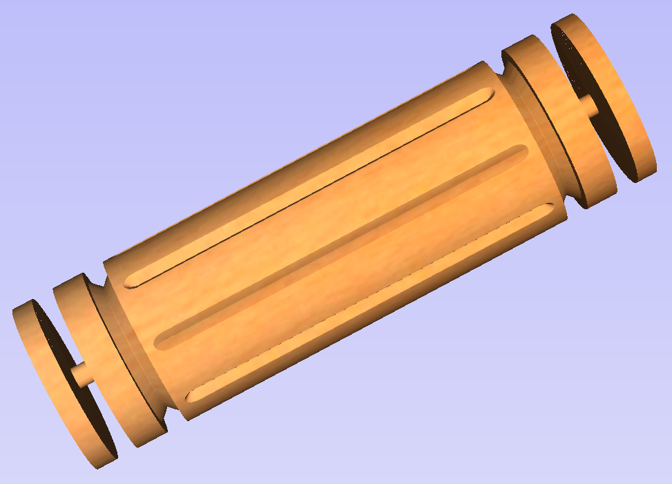
Although the design can be considered to be finished, in practice it is useful to be able to cut-out the remaining stock. This can be realized by making the design slightly longer and adding profile cuts. In this example the blank length was extended by 2 inches using the Job Setup . Existing vectors can be recentered using F9After that the existing toolpaths have to be recalculated.
The cut-out vectors can be created in the same way as cove vectors. Two extra profiling toolpaths can be created using the suitable End Mill. In this example we used a tab with a 0.5 inch diameter. In order to achieve that, the user can type the following in the Cut Depth box: z-0.25 and then press = and the software will substitute the result of the calculation. Variable 'z' used in the formula will be substituted by the radius of the blank automatically by software. It is also important to specify Machine Vectors Outside/Right or Machine Vectors Inside/Left as appropriate. The cut-out toolpaths and the resulting simulation can been shown below.
The final step is to save the toolpaths in a format acceptable by your machine. Use the Save Toolpaths and select the wrapped post-processor matching your machine.
Note
Tools and values presented in this example are for illustrative purposes only. Size of tools, feed rate, tabs diameter etc. have to be adapted to the material and machine used to ensure safe and accurate machining.
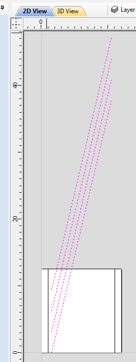
Spiral toolpaths
This section will explain how to create and simulate spiral toolpaths.
One way of thinking about spiral toolpaths is to imagine a long, narrow strip of fabric. Such a strip can be wrapped around a roll at a certain angle. In order to create a toolpath that wraps around the blank multiple times, one can create a long vector at a certain angle. Such a vector is an equivalent to the strip of fabric when it is unwrapped from the roll.
Although such a toolpath will exceed the 2D workspace of the rotary job, thanks to the wrapping process during both simulation and machining the toolpath will actually stay within material boundaries.
The most crucial part of designing spiral vectors is to determine the right angle and length of the line that would result in a given number of wraps. Suppose one would like to modify a simple column design to use spiral flutes, rather than parallel to rotation axis. The following example will use flutes wrapping 3 times each, but the method can be adapted to any other number.
All but one of the existing flute vectors can be removed. Select the Draw Line/Polyline and start a new line by clicking at one end of the existing flute. This line needs to be made along the wrapped axis with the length being 3 times the circumference of the job. In this example that means typing 90 into the Angle box and typing y * 3 into the Length box and pressing =. If the wrapped axis is not the Y axis, but rather the X axis, then the above formula should be x * 3.
Now one can simply draw a line connecting to the other end of the original flute vector and the newly created one. Using Copy Along Vectors tool this single flute may be copied in the way described earlier. In this example 4 spiral flutes were created, as can be seen below.
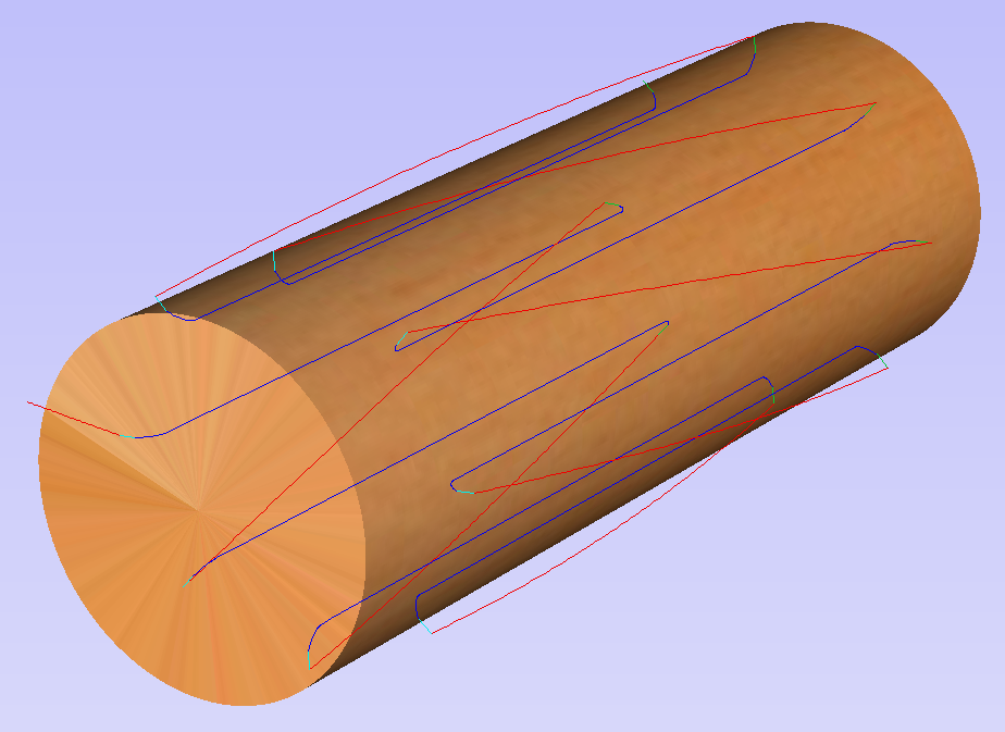
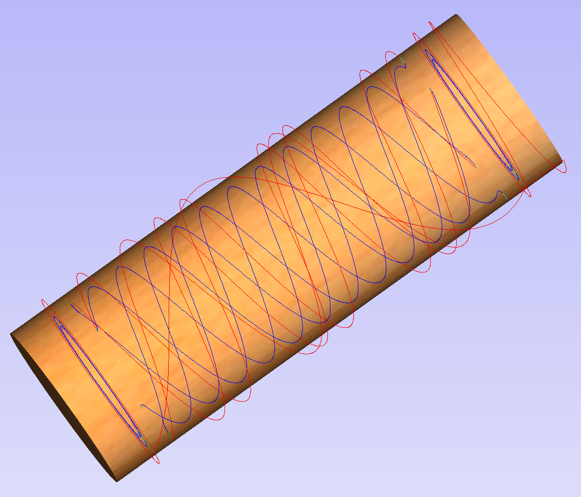
Once the flute vectors are ready, the toolpath can be created again using the Fluting Toolpath. An important thing to note, is the difference between the appearance of spiral toolpaths in the wrapped and flat view. By clicking on Auto Wrapping one can switch from wrapped rotary view to flat view and back again.
As can be seen above, in the flat view the toolpaths will follow the vectors and extend beyond the job boundaries. On the other hand the wrapped view, presented below, will display the toolpaths spiralling around the blank.
This was just a brief overview of general 2D workflow for rotary machining. Remember to also take a look at video tutorials dedicated to rotary machining, which are accessible from the Tutorial Video Browser link when the application first starts.
Modelling 3D Rotary Projects
Elaborating 2D designs with 3D clipart pieces
This section will present how to add 3D clipart to basic fluted column presented in Simple rotary modelling using 2D toolpaths.
A simple way to start with 3D rotary models is to use add pieces of decorative clipart that is provided with Aspire. This process is very similar to adding clipart to single - or double - sided project, however there are some additional considerations that are specific to wrapped rotary machining.
To start, switch to the Clipart tab. Then choose a piece of clipart and drag and drop it into the workspace. Aspirewill show following message:
To understand this message, we need to consider the flat view of our model, after importing the clipart. Flat view can be accessed by clicking Auto Wrapping button.
As can be seen, the model contains only the selected decorative piece on the flat plane. Although the column is obviously a cylindrical solid, so far we only used 2D toolpaths to carve details on the surface of cylinder. So the fact that machined piece is a cylindrical solid, derives only from fact that the blank is a cylindrical solid itself. Aspireallows the 3D model to also describe a solid body.
In this example the intent is to only place a decorative piece on the surface, rather than define body of the column. Aspirecan see that we did not model a body and we are placing a piece of clipart, that is likely to be placed at the surface. By responding 'Yes' to the message we can confirm that it is our intent to use the component to decorate a surface.
Note
The above message is only displayed when the 3D model is empty. Regardless of user choice, this message will not be displayed again for this project.
More clipart can be placed as desired. Then the 3D view can be inspected. Once design is finished it is time to create toolpaths. In order to create 3D roughing toolpath, use the 3D Roughing Toolpath. Then create 3D finishing toolpath, using 3D Finish Toolpath. Select settings that are most appropriate for given application, while remembering which axis is rotating. The choice of axis may be particularly important if rotation axis speed is slower than linear axis.
In this example the decorative clipart that was added was not recessed. That means that after 3D machining the flat areas around clipart will be recessed due to clipart 'standing out' of the flat surface. Therefore existing 2D toolpaths needs to be projected. This can be accomplished by selecting Project toolpath onto 3D model option and recalculating the toolpaths.
Making a tapered column
This section will explain how to make a tapered column by modifying the basic design from previous section.
So far only the surface details were modelled. In order to make a tapered shape, we need to model 'body' of the shape in addition to surface details. For that purpose, zero plane component can be used. It is added automatically for rotary jobs.
Double-click the zero plane component to open Component Properties. Enter 0.8 in the Base Height box. Select Tilt option. Click Set button in Tilt section, then switch to 2D view and then click in the middle left and then in the middle right. Set the angle to 3 degrees.
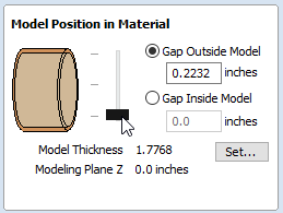
Since the modelling plane was adjusted for placing component on the surface, it needs to be adjusted again, so the component body is not 'inflated'. To do that open the Material Setup form. Adjust modelling plane by moving the slider down, until the Gap Inside Model is 0.
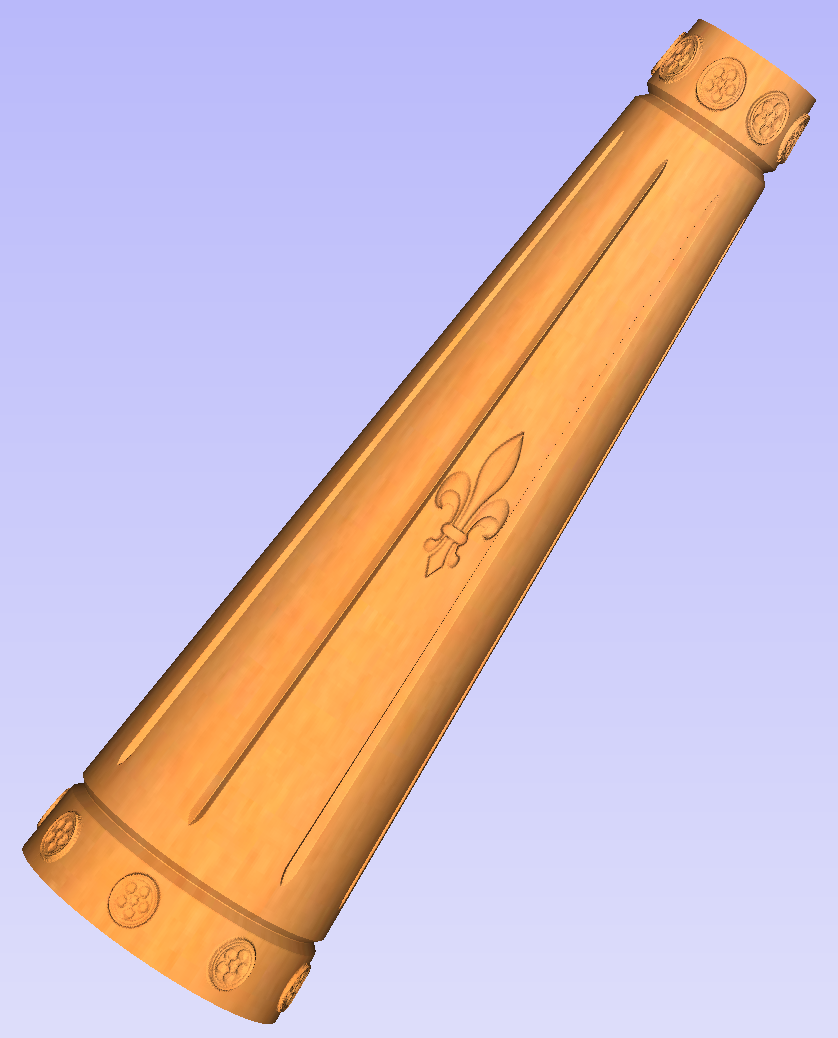
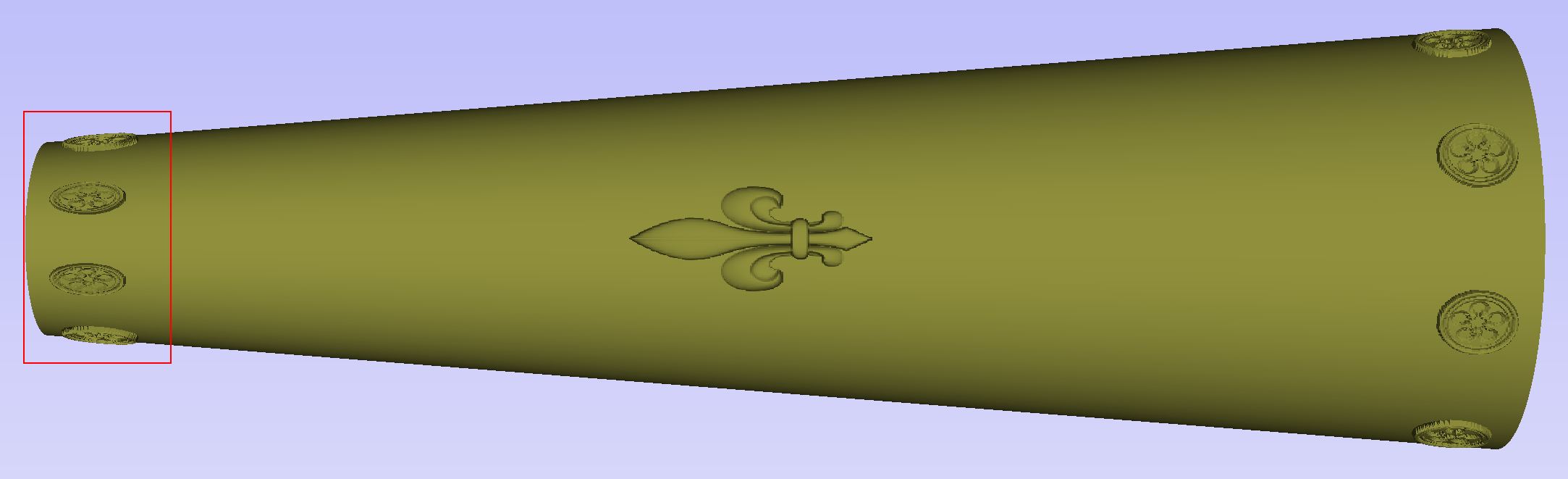
After modelling a tapered shape, the 3D model of column will have a desired shape. However clipart pieces in the narrower parts have been distorted, as can be seen below. To fix that, one needs to stretch the components in the wrapped dimension, to compensate for distortion.
The distortion that has been demonstrated above, applies also to toolpaths. That means that wrapped toolpaths will match flat toolpaths only at the surface of the blank. The closer to the rotation axis (i.e. deeper) the toolpath is, the more it will be 'compressed'. This fact have a profound implication for 3D toolpaths. Consider the example shown below.
As can be seen if there is substantial difference in diameter in different parts of model, generating one 3D toolpath for whole model will result in wrapped toolpath being overly compressed. Thus it is usually better to create boundaries of regions with significantly different diameter and generate separate toolpaths using correct settings for each diameter.
Modelling turned shapes
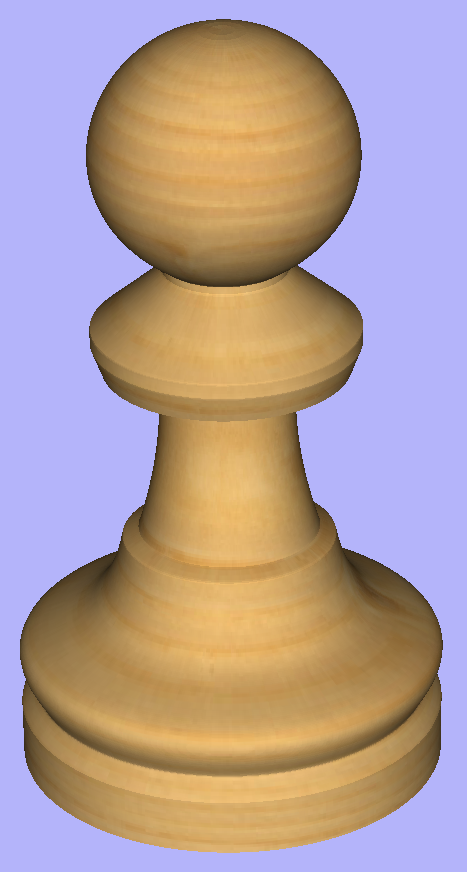
This section will present a basic technique for creating turned shapes.
Modelling turned shapes is quite easy. It requires a vector representing a profile of the desired shape and a Two Rail Sweep tool.
To start, create a new rotary job. Then either draw a profile using available drawing tools or import profile vector. This example used a chess pawn profile, as can be seen below.
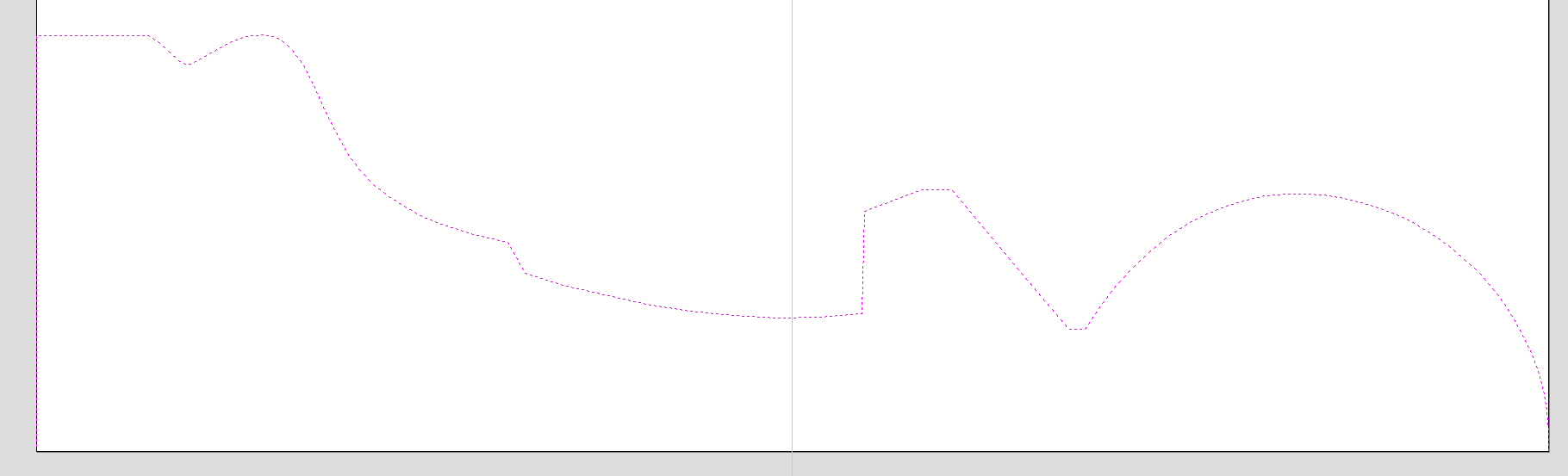
Open the Two Rail Sweep tool. When the rotary job is created, the software inserts a special layer called '2Rail Sweep Rails'. It contains two blue lines on the sides of the job, that are perpendicular to the rotation axis.
Select both of those rails and click the Use Selection button. The rails will then be highlighted. Then select the profile vector and click apply. Inspect the 3D view to verify the results.
Modelling cross section
This section will explain how to model desired shape using Vector Unwrapper.
The Vector Unwrapper is useful when rather than modelling a profile along the rotation axis, it is more intuitive to specify a desired cross section. The tool transforms a vector, representing a cross section, into a profile vector that can be subsequently used with Two Rail Sweep tool.
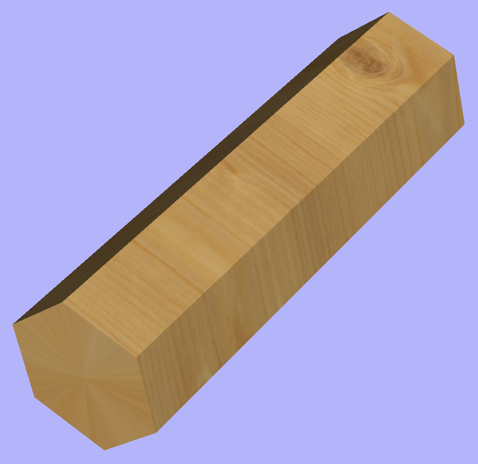
Suppose we would like to create a hexagonal-shaped column. Let's start by creating a new rotary job. In this example job has a diameter of 6 inches and is 20 inches long. X axis is the rotation axis and Z origin has been placed on the cylinder axis.
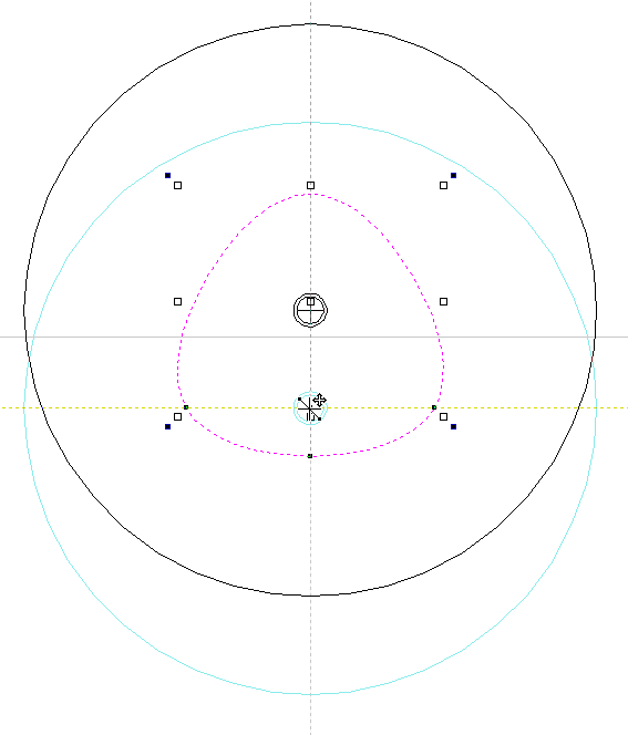
We need to create a hexagon using Draw Polygon tool. This vector will serve as a cross section and can be placed anywhere in the 2D view. In this example the material block diameter is 6 inches, so the radius of the shape cannot exceed 3 inches.
When the shape is created, select it and open Vector Unwrapper. The tool will display a crosshair in place where the rotation axis is crossing the profile and a circle with the diameter of the material block. This will help you determine whether the shape with such cross profile will fit in current material block.
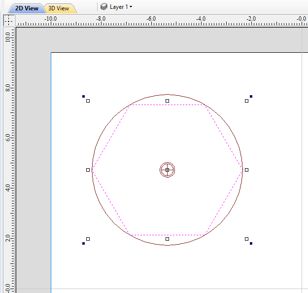
In this example, the Use Center of contour option was used. That means that rotation axis will be placed in the centre of vector's bounding box. One can also tick Simplify unwrapped vectors option to fit bezier curves, instead of using series of very short line segments. After apply is pressed, the unwrapped version of the selected cross section will be created, as have been shown below.
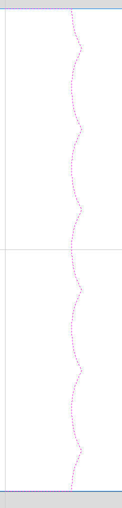
This example shows the unwrapped vector for a cylinder rotating around the X axis. If your rotary axis is aligned along Y the unwrapped vector will be horizontal. It is worth noting that unwrapped profile have 'legs' on each end. Those are needed to ensure that correct height will be used in the next step.
The tool automatically creates layer called 'Unwrapped Vectors Drive Rails' on which it places two blue line vectors on job sides, parallel to the rotation axis. In order to extrude the profile, open the Two Rail Sweep tool. Then select top and then bottom rail (left and right when Y axis is rotation axis) and confirm selection by clicking Use Selection button. The rails will now be highlighted. Now click on unwrapped vector and press apply. The 3D view will show a hexagonal column, that can be seen at the beginning of this section.
Modeling Plane
The desired cross-section will only be achieved if modelling plane is positioned in cylinder centre. That means that Gap Inside Model is reported as 0 in Material Setup form. Otherwise the resulting model will have incorrect diameter and the cross section will become rounded.
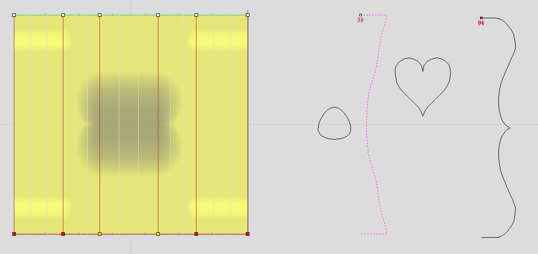
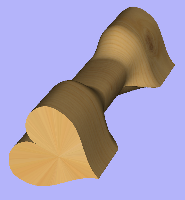
The Vector unwrapper is not restricted to simple shapes. In principle it is always possible to use convex shapes and certain concave shapes. The example below shows a heart profile unwrapped.
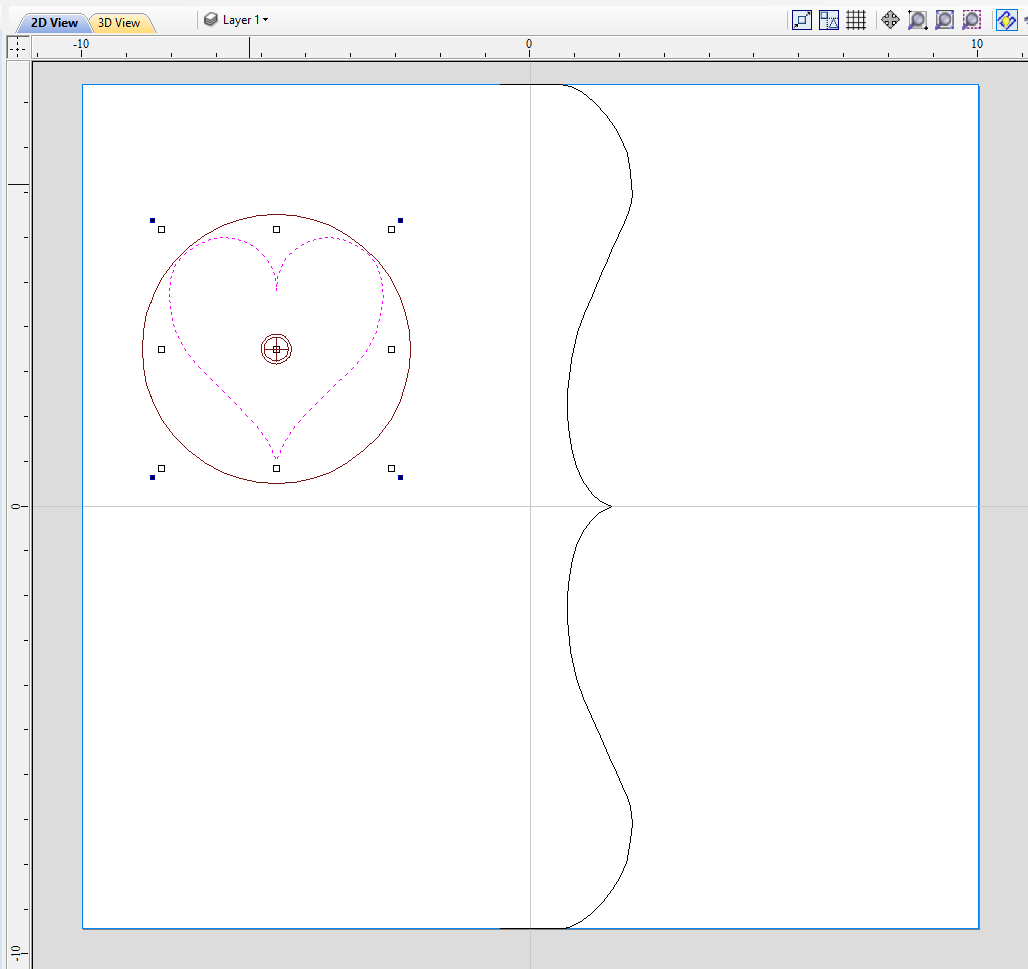
If cross section in question is concave, one could imagine straight line starting in the center of the shape and touching a point on the boundary. If the second points keeps travelling along the boundary and each line is not crossing another point on the boundary, then it is possible to use this cross section. If the line does cross more than one point on the boundary, this part of the cross section will not be represented correctly.
All the examples so far used a single cross section. However it is also possible to use multiple cross sections.
Let's take another cross section and open Vector Unwrapper. Then drag the rotation axis handle a bit down from the center. If snapping is enabled, it can be used to help position the rotation center, as can be seen below.
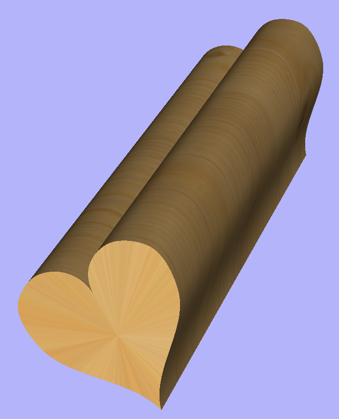
Once we have another unwrapped cross section, it is possible to use both during Two Rail Sweep. For example unwrapped heart profile can be placed twice on the left and twice on the right. The second unwrapped profile can be placed twice in the middle. Such arrangement may result in shape morphing, as can be seen below.
Advanced Modelling of 3D Rotary Projects
Modelling 3D spiral features
In this section we will show how to use level-wrapping feature to wrap a design in spiral manner around a column.
The workflow for creating spiral toolpaths has been presented in the Simple rotary modelling using 2D toolpaths chapter. The basic idea involved creating a line at a proper angle to the rotation axis, that exceeded the 2D boundaries. When 2D toolpath is created based on such a line, it will be wrapped around material cylinder, creating a spiral.
This guide will build on that basic idea. The task is to create a horizontal strip with desired pattern and then wrap it like a ribbon around the cylinder.
To help with that task, it is important to create some helpful vectors first. We need to create lines, that will become boundaries of our strip. In this example the strip was being wrapped four times around full length of material. This example assumes that rotation axis is parallel to X axis.
To start, select Draw Line/Polyline tool and draw a horizontal line at the bottom of the job from left to right. If it is desired for the spiral pattern to only fill part of the cylinder length, this horizontal line should be drawn only in th desired location. While the drawing tool is still active, type 90 into Angle box and type y * 4 into Length box and pressing =. We used y * 4 formula so the strip will wrap 4 times. Then press Add button to add a vertical segment.
Now, start a new line that connects the horizontal and vertical lines, forming a triangle. Once this line is created, horizontal and vertical lines can be removed.
The line that we just created will form a bottom of the strip. Now copy this line and place line so its bottom left end coincides with top left corner of the 2D job. This line will form a top of the strip. Then make another copy and place it in the middle. This middle line will be used later to position our design within strip. All three lines have been shown below.
Next step is to find out the required length and width of the strip. We will need a few extra vectors to accomplish that.
Let's copy one of the created three lines and rotate by 90 degrees, to get a line that is perpendicular to the strip. Then place it in such way so it crosses the strip. This will help us measure the width.
Then copy the perpendicular line and place it so it touches the top line. Then extend the bottom line, until it crosses the perpendicular line we just added. This will help us measure the length of the strip.
The easiest way to achieve that, is to create a textured component. To do that, select the design in the component tree and activate the Create Texture Area tool. This example used the default settings of the tool. The tool will create a new component that will fill the whole 2D job boundaries. The component itself will be filled with the design in tiled manner. Now use the Set Size tool to resize textured component to match the strip size.
Now the component have to be rotated and moved to fit between the lines you have drawn at the beginning. This process can be made easier by utilizing Copy Along Vectors tool. To proceed, activate the tool and select the textured component first, then select the middle line in the strip while holding Shift. Make sure that Align objects to curve option is selected and use Number of copies option. Since our strip has already have a correct size, we only need one copy. However the tool would place the middle of our component at the beginning of the line only. If you enter 3 as the number of copies, then the tool will place two copies of component at each end and in the middle. Afterwards the copies at the ends can be simply deleted. The picture below shows the strip in the 3D view after being correctly positioned.
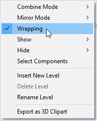
As can be seen, the strip disappears as soon as it leaves the material boundaries. In order to make it wrap around, we need to create a new level in the component tree and move the texture component into it. Then right click on the newly created level and right click. From the pop-up menu select wrapping. After that wrapping will occur.
Note:
Wrapping can be enabled on any level in component tree and combined with mirror mode. If the level wraps on itself, then intersecting areas will be merged regardless of level's combine mode. If it is desired to create e.g. a woven pattern, then place left-hand spiralled component and right-hand spiralled components in different separate levels, both with wrapping enabled.
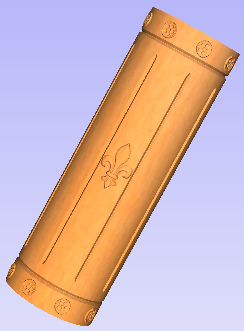
The last step is to make column endings. For that purpose the third level was created, with Combine Mode set to Merge. This way the spiral pattern will be 'hidden' at the ends. A circular 3D tab clipart was placed at each end, and stretch vertically to match the job boundaries.
Modelling twisted shapes
This section will show how to create twisted shapes, using a combination of level-wrapping and Vector Unwrapper tool.
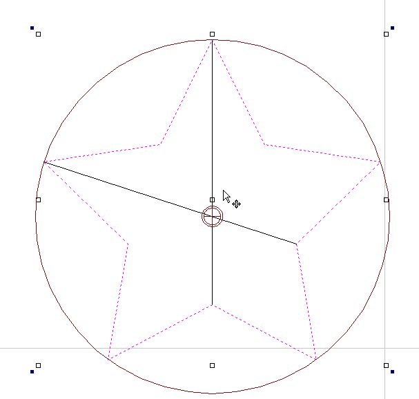
In this example a new rotary job was created, with a diameter of 6 inches and length of 20 inches, rotating around X axis. To start, we need a cross-section vector. In this example a 5-armed star was used. To create a star, we can use Draw Star tool. This example used Outer Radius of 3 inches, to match the radius of the material.
The next step is to unwrap the cross section. In the case of the star however, the center is not the same as center of star's bounding box. To find the real center, one can draw a line from two of the star corners. Then open Vector Unwrapper and select the star. Then drag rotation center and snap it to the intersection of the lines, as can be seen below.
Once the star is unwrapped, we need to create rails, that will make spiral when wrapped. To do that, select Draw Line/Polyline tool and draw a horizontal line at the bottom of the job from left to right. While the drawing tool is still active, type 90 into Angle box and type y * 2 into Length box and pressing =. We used y * 2 formula so the star will make 2 revolutions Then press button to add a vertical segment. Finally, start a new line that connects the horizontal and vertical lines, forming a triangle. Once this line is created, our horizontal and vertical lines can be removed.
Next step is to copy the line and place it so its bottom left end coincides with top left corner of 2D job.
Once the the rails are ready, one could use a Two Rails Sweep tool. However, since rails exceeds the 2D job boundaries, the created sweep will be cropped as soon as those boundaries are exceeded.
To overcome that, select both rails, open Draw Rectangle tool and press . This will create a bounding box containing the rails. Now, write done the size of the box and save current project. Then create a new single-sided project with the slightly bigger than the bounding box. Use the Import Vectors option from the main menu and select the previously saved file. Now select the rails and press F9 to center them.
Now use Two Rail Sweep tool. When component is ready, save the file.
Now re-open the original rotary project. Use Import Component and select the single-sided project created in the step above. Move the component to the desired location. Then, create a new level, move the component there and enable wrapping.
Using single-sided modelling tools
This section will present how to use single-sided modelling techniques in rotary projects.
Users familiar with modelling techniques used in single-sided projects may find them more convenient for modelling certain shapes. This example uses two vectors, representing side cross section of the table leg and a few of half cross sections for different parts of the table leg. Those vectors are presented below.
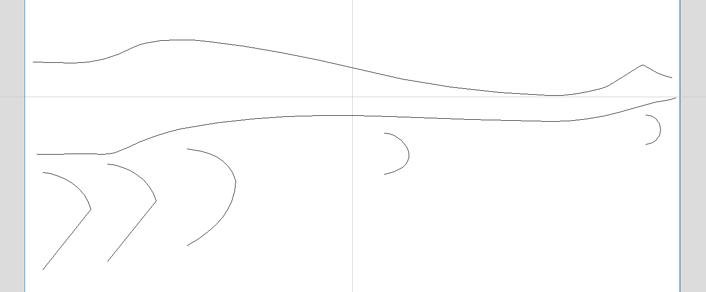
One can simply treat the side cross section as rails and use the Two Rail Sweep tool, placing the half cross sections at appropriate locations. This way half of the leg can be modelled very quickly, with the result that can be seen below (using flat 3D view).
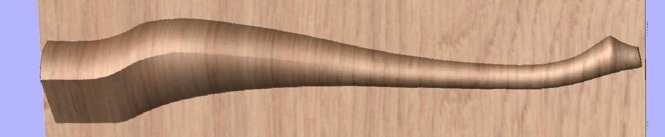
In order to use the created model in a rotary project, we need to export and then import it back. Although it is possible to do this with two sessions of Aspire, it can also be done within a single session with rotary project. To export the leg model, make sure no other components are visible (including the automatically added zero plane) and open the Export Model tool while holding down Shift. Pressing Shift allows to open the export tool in single-sided, rather than rotary mode.
Since half of the leg was modelled, Close with inverted front option can be used. The resulting STL mesh can be seen below.
Once component is exported, it can be re-imported as Full 3D model. The model will have a seam, in the place were two halfs were merged. This can be removed using smoothing function of the Sculpting tool.
ポストプロセッサ編集
ポストプロセッサの用途
ポストプロセッサとは、特定のルーターまたは工作機械に対して適切な形式に、工具移動のXYZ座標を変換するプログラムのセクションです。
構成ファイルは、特定のマシンコントロールに適応するように、プログラムからの出力をカスタマイズします。このドキュメントは、構成ファイルの作成および編集方法の詳細を説明します。
以下は、G-CodeとHPGLにポストプロセスされた一般的なプログラムのセクションを示します。
G-Code出力
T1 M6
G17
G0 Z4.5000
G0 X0.0000 Y0.0000 S12000 M3
G0 X2.4567 Y7.8342 Z0.2500
G1 Z-0.0500 F5.0
G3 X3.3784 Y8.7559 I0.0000 J0.9218 F66.0
G3 X2.4567 Y9.6777 I-0.9218 J0.0000
G3 X1.5349 Y8.7559 I0.0000 J-0.9218
HPGL出力
IN;PA;
PU2496,7960;
PD2496,7960;
AA2496,8896,90.000
AA2496,8896,90.000
AA2496,8896,90.000
AA2496,8896,90.000
PU2496,7960;
PU2496,6096;
マシンコントローラーの製造元は、特定のマシンで実行するためのプログラムに必要な形式に、ファイルをカスタマイズする場合があります。これにより、当該マシンの特性に適応するように、コントロールを最適化することができます。
Vectricのポストプロセッサは、簡素なテキストベースの構成ファイルを使用します。そのため、必要に応じて、ユーザーによる構成ファイルのカスタマイズが可能です。
ポストプロセッサの各セクション
Vectricのポストプロセッサは、明瞭性の観点から複数のセクションに分類されているので、類似したスタイルで独自のポストプロセッサを書き出して、デバッグに利用することができます。
ファイルコメント
ポストプロセッサの説明や、ポストプロセッサへの変更を記録するセクションです。「+」または「|」文字で開始される各行が、コメントとなります。
+ 履歴
+ 日時、担当、作業
+ ======== ========== ===========================
+ トニー 14/07/2006 書き出し
+ マーク 26/08/2008 ATCコマンド結合、TCでスピンドル停止
+================================================
グローバルファイルステートメント
ステートメントとは、一度だけ使用されるアイテム、または、ファイルを通じて複数の静的な値を持つアイテムです。明瞭性を保つために、ステートメント名には大文字のみを使用します。
ステートメント | 結果 |
|---|---|
| ポストプロセッサのリストに表示される名前です。 |
| ファイルに与えられるファイル拡張子です。 |
| ファイルが出力する単位(インチ/MM)です。 |
| 工作機械の製造元は、NCファイル出力の直接受け入れが可能なドライバー(通常はプリンタードライバー)を提供します(例: Generic HPCL_Arcs.pp参照) |
| (素材設定フォームで指定される)Plunge (Z2) 高さへの切り込み動作が、早送り移動であることを示します。 |
| コントロールソフトウェアが、NCファイル出力の直接受け入れが可能なドキュメントインターフェイスを使用します。 |
| Y軸の移動が、指定された直径の円筒周りにラップされます。「Y」値は「A」として出力されます。 |
| X軸の移動が、指定された直径の円筒周りにラップされます。「X」値は「B」として出力されます。 |
| 当該マシンの回転速度は、スピンドルの実際の速度(RPM)を表す1から15までの整数の範囲として出力されます(この例では、4500から15000 RPM)。 |
| このコマンドを使用して、( 文字は「オリジナル - 代用」のようにペアで入力されます。 例えば、MACH 3コントロールソフトウェアは、コンマ区切りとして丸括弧を使用し、ネスト化されたコメントの利用は許容しません。 |
| Rotary: 逆時間送りモードにおける送り速度Fの出力の有効/無効を切り替えます。 GCodeでは、これによりG93がオンになるかG94がオフになり、単位モードを使用します。 |
| 当該ポストプロセッサが、レーザー工具経路をサポートすることを示します(レーザーモジュールがインストール済みの場合)。 |
| 任意の最小円弧半径です。この値より小さな半径を持つ円弧は、単一の直線移動に変更されます。 |
| 任意の最大円弧半径です。この値より大きな半径を持つ円弧は、ポリゴン化されます。 |
テープ切り離しサポート
工具経路の出力が分割される長さを説明します。
TAPE_SPLITTING=MAX_NUM_LINES LINE_TOL "FILENAME_FORMAT" START_INDEX INDEX_ON_FIRST_FILE
以下のコマンドを例として使用します。
TAPLE_SPLITTING=1000 100 "%s_%s.tap" 1 "YES"
この場合
出力は最大1000行(ただし、その多くの行がポストプロセッサのフッターセクション内)の複数ファイルに分割され、900行(1000 – 100)以降にリトラクト動作がある場合、ファイルは該当する移動で分割されます。ファイル名が「toolpath」の場合、分割されるファイルの名前は「toolpath_1.tap」、「toolpath_2.tap」となります。最初の工具経路出力は、「toolpath_ 1.tap」となります。 INDEX_ON_FIRST_FILE= YES が使用されているため、「toolpath」はインデックス番号なしにはなりません。ただし、ファイルが1000行未満の場合はファイルが分割されないため、この限りではありません。
注記
NCファイルの分割が必要な一部のコントローラーでは、ファイル名の文字数にも制限があります。例えば、MSDOSスタイルの8.3ファイル名形式での命名が必要になる可能性があります。出力ファイルの命名時には、この点を考慮する必要があります。
行終了文字
LINE_ENDING="[13][12]"
文字の10進数値は、ポストプロセッサファイルの各個別行にアペンドされます。WindowsまたはMSDOS形式のテキストファイルの読み込みが可能なコントローラーでは、通常は[13][10](復帰、改行)となります。
ナンバリングのブロック
出力ファイルに行番号を追加する場合、現行行番号が変数[N]で追加されます。この行番号変数の挙動は、以下の変数に制御されます。
ステートメント | 結果 |
|---|---|
| 行番号を開始する値です。 |
| 行番号間の増分値です。 |
| 再度 重要:一部のコントローラーでは、コントロール上に表示可能な行数に制限があります。 |
変数
変数名 | 以下で出力 | 値 | サンプルファイル |
|---|---|---|---|
|
| 現行送り速度です。 | Mach2_3_ATC_Arcs_inch.pp |
|
| 現行加工送り速度です。 | CNCShark-USB_Arcs_inch.pp |
|
| 現行切り込み送り速度です。 | CNCShark-USB_Arcs_inch.pp |
|
| R.P.Mの現行回転速度です。 | GCode_arc_inch.pp |
|
| JETベースの工具(レーザーなど)の現行電源設定です。 | grbl_mm.pp |
|
| 現行工具番号です。 | Mach2_3_ATC_Arcs_inch.pp |
|
| 前の工具番号です。 | NC-Easy.pp |
|
| 行番号です。 | Mach2_3_ATC_Arcs_inch.pp |
|
| 現行工具名です。 | MaxNC_inch.pp |
|
| 現行工具のToolDBのメモフィールドからのテキストです。 | Busellato_Jet3006_arc_inch.pp |
|
| 現行工具経路名です。 | Viccam_ATC_Arcs_inch.pp |
|
| (「工具経路保存」に生成される)ファイル名です。 | ez-Router_inch.pp |
|
| 工具経路ファイルの保存先フォルダーです。 | Woodp_arc_mm.pp |
|
| 工具経路のファイル拡張子です。 | TekcelE_Arc_ATC_3D.pp |
|
| 工具経路のフォルダーパス名です。 | WinPC-NC_ATC_Arcs_mm.pp |
|
| X軸における工具位置の現行座標です。 | GCode_arc_inch.pp |
|
| Y軸における工具位置の現行座標です。 | GCode_arc_inch.pp |
|
| Z軸における工具位置の現行座標です。 | GCode_arc_inch.pp |
|
| A軸における工具位置の現行座標です。 | |
|
| X軸における円弧の中心です(最終X,Y位置に相対)。 | Mach2_3_ATC_Arcs_inch.pp |
|
| Y軸における円弧の中心です(最終X,Y位置に相対)。 | Mach2_3_ATC_Arcs_inch.pp |
|
| X軸における円弧の中心です(絶対座標)。 | Isel_arc_mm.pp |
|
| Y軸における円弧の中心です(絶対座標)。 | Isel_arc_mm.pp |
|
| X軸における円弧の開始位置です。 | TextOutput_Arcs_mm.pp |
|
| Y軸における円弧の開始位置です。 | TextOutput_Arcs_mm.pp |
|
| Xにおける円弧の中点です(絶対座標)。 | TextOutput_Arcs_mm.pp |
|
| Yにおける円弧の中点です(絶対座標)。 | TextOutput_Arcs_mm.pp |
|
| Xにおける円弧の中点です(増分座標)。 | TextOutput_Arcs_mm.pp |
|
| Yにおける円弧の中点です(増分座標)。 | TextOutput_Arcs_mm.pp |
|
| 円弧の半径です。 | Bosch_ATC_Arcs_mm.pp |
|
| 円弧の角度です。 | Generic HPGL_Arcs.pp |
|
| X軸のホーム工具位置です。 | CAMTech_CMC3_mm.pp |
|
| Y軸のホーム工具位置です。 | CAMTech_CMC3_mm.pp |
|
| Z軸のホーム工具位置です。 | CAMTech_CMC3_mm.pp |
|
| 安全高さ/早送りクリアランス間隔です。 | EMC2 Arcs(inch)(*.ngc) |
|
| 軸がラップされる円筒の直径です。 | Mach2_3_WrapY2A_ATC_Arcs_mm.pp |
|
| Xにおける素材の長さです。 | Mach2_3_ATC_Arcs_inch.pp |
|
| Yにおける素材の長さです。 | Mach2_3_ATC_Arcs_inch.pp |
|
| Zにおける素材の長さです。 | Mach2_3_ATC_Arcs_inch.pp |
|
| Xにおける素材の最小値です。 | MaxNC_inch.pp |
|
| Yにおける素材の最小値です。 | MaxNC_inch.pp |
|
| Zにおける素材の最小値です。 | MaxNC_inch.pp |
|
| Xにおける素材の最大値です。 | MaxNC_inch.pp |
|
| Yにおける素材の最大値です。 | MaxNC_inch.pp |
|
| Zにおける素材の最大値です。 | MaxNC_inch.pp |
|
| Xの原点位置です。 | TextOutput_Arcs_mm.pp |
|
| Yの原点位置です。 | TextOutput_Arcs_mm.pp |
|
| Zゼロ位置、テーブルまたは素材サーフェスです。 | TextOutput_Arcs_mm.pp |
|
| X,Y原点です。 | TextOutput_Arcs_mm.pp |
|
| 使用された工具のリストです(使用順)。 | Mach2_3_ATC_Arcs_inch.pp |
|
| ファイルで使用された工具経路のリストです(使用順)。 | Mach2_3_ATC_Arcs_inch.pp |
|
| 工具経路のメモです(工具経路設定フォーム)。 | Mach2_3_ATC_Arcs_inch.pp |
|
| ファイルのメモです(編集 > メモ)。 | Mach2_3_ATC_Arcs_inch.pp |
|
| ファイル作成時間です。 | Mach2_3_ATC_Arcs_inch.pp |
|
| ファイル作成日です。 | Mach2_3_ATC_Arcs_inch.pp |
|
| 穴あけ加工時のドウェル時間(秒)です。 | Mach2_3_Arcs_inch.pp |
|
| ファイルの出力に使用された製品名です(バージョン番号含む)。 | |
|
| 工具直径です。 | |
|
| Rotary: 現行の逆時間レートです。 | AvidCNC_WrapX2A_G93_inch.pp |
変数の形式
工具位置の値、送り速度、回転速度などは、変数を使用してファイルに挿入されます。ファイル全体で変数が使用されます。ファイルのポストプロセスが行われると、変数が当該アイテムの現行値で置換されます。
例えば、変数出力の[X]、[Y]、[Z]をそれぞれ使用して、いつの時点でも現行のXYZ工具位置がファイルに挿入されます。
明瞭性を保つために、変数名には大文字のみを使用します。
変数は以下のようにフォーマットされます。
VAR VARIABLE = [VO|WO|CS|VF|MX]
この場合
VO= X、XF、Fなどの変数出力です。WO= 出力がA=常時、C=変更時のみ行われます。CS= 文字列が値の前に出力されます。VF= 値が出力される形式を指定する値の形式です。MX= 乗数値です。
一般的な変数
1 | 2 | 3 | 4 | 5 | 6 | 7 | 8 | 9 | 10 | 11 | 12 | 13 | 14 | 15 |
|---|---|---|---|---|---|---|---|---|---|---|---|---|---|---|
|
|
|
|
|
|
|
|
|
|
|
|
|
|
|
VAR- この行は変数です。- 変数名です。
- 等号です。
- 開始角括弧 - 変数フォーマットパラメーターの開始です。
- 変数ラベル - 変数値で代用されるラベルです。
- 縦棒 - パラメーターの区切りです。
A= 常に値を出力、C= 変更時のみ値を出力することを表します。- 縦棒 - パラメーターの区切りです。
- 変数値の前に印刷するための文字列です。
- 縦棒 - パラメーターの区切りです。
- 任意のフォーマットフラグ - (後述)。
- 値の形式 - 出力する単位と小数点以下の桁数です。
- 縦棒 - パラメーターの区切りです。
- 出力乗数 - (後述)。
- 終了角括弧 - フォーマットパラメーターの終了です。
出力値のフォーマット
値フォーマット文字列は、以下のようにフォーマットする必要があります。
FORMAT_FLAGS FIELD_WIDTH DECIMAL_SEPARATOR DECIMAL_PLACES
フォーマットフラグは任意で、後述するごく一部のコントローラーのみに必要です。
フィールド幅:出力される最少数の文字を表します。通常、フィールド幅は「1」に設定されます。それより大きな値は、コントローラーが値に対して固定数の文字を求める場合のみ必要になります。そのような場合には、1より大きな値を入力することができます。入力された値の文字数が、確実に出力されるようになります。フィールド幅を表す数値は、出力値の完全な浮動小数点(小数点記号)を含みます。
小数点:小数点記号は、ほとんどの場合でピリオドが使用されますが、一部のコントローラーではコンマが使用される場合があります。(ピリオドを使用しないポストプロセッサの例として、以下のファイルを参照してください。Heidenhain_inch.pp)
小数点位置:出力される小数点以下の桁数です。多くの場合で、メトリック法で操作されるコントローラーには3、インチ法のコントローラーには4が設定されます。
任意のフォーマットフラグ
出力値は、任意のフォーマットフラグを使用してさらに修正可能です。
フラグ | 機能 | デフォルト(フラグなし) |
|---|---|---|
| 値は右端に揃えられます。 | 値は右端に揃えられます。 |
| 値に「+」または「-」接頭辞を付けます。 | 値に「+」または「-」接頭辞を付けます。 |
| 値が設定された最小値未満の場合、値に接頭辞「0」を付けます。 | 値には空のスペースである接頭辞が付けられます。 |
| 値は常に区切り文字付きで出力されます(実際には、値が整数値のみを出力するように設定される場合に限り、出力値を変更します)。 | 出力が整数のみに設定されると、区切り文字は値にアペンドされません。 |
変数のデフォルトフォーマット
多くの変数にデフォルトの形式があります(以下参照)。変数に対して別の形式を設定するには、ポストプロセッサに以下の行を入力し、使用するコントローラーに適したパラメータに変更します。
デフォルト | サンプル |
|---|---|
|
行番号は常に出力されます。「N」文字が行番号の前に挿入されます。整数として出力されます。 |
|
回転速度は常に出力されます。「S」文字が値の前に挿入され、整数として出力されます。 |
|
送り速度は値の前に「F」文字で出力され、変更時のみ出力されます。値は小数位1桁まで出力されます。 注記 このフォーマット文字列では、任意の追加パラメーターがあります。これは値乗数です。 |
VAR PLUNGE_RATE = [FP|A||1.0] |
切り込み速度は値の前に「F」文字で出力され、変更時のみ出力されます。値は小数位1桁まで出力されます。 注記 このフォーマット文字列では、任意の追加パラメーターがあります。これは値乗数です。 |
|
加工速度は値の前に「F」文字で出力され、変更時のみ出力されます。値は小数位1桁まで出力されます。 注記 このフォーマット文字列では、任意の追加パラメーターがあります。これは値乗数です。 |
|
位置値は値の前に「X」文字で出力され、位置は常に出力されます。また、一般的にはメトリック法の出力を必要とするコントロールに適した小数位3桁まで出力されます。 インチ法で操作されるコントローラーには、通常小数位4桁まで値を出力します。以下のように行をフォーマットします。
|
|
ホーム位置値は値の前に「X」文字で出力され、位置は常に出力されます。また、一般的にはメトリック法の出力を必要とするコントロールに適した小数位3桁まで出力されます。 インチ法で操作されるコントローラーには、通常小数位4桁まで値を出力します。以下のように行をフォーマットします。
|
|
値は値の前に「X」文字で出力され、位置は常に出力されます。また、一般的にはメトリック法の出力を必要とするコントロールに適した小数位3桁まで出力されます。 インチ法で操作されるコントローラーには、通常小数位4桁まで値を出力します。以下のように行をフォーマットします。
注記 このフォーマット文字列では、任意の追加パラメーターがあります。これは値乗数です。 |
|
値は値の前に「Y」文字で出力され、値は常に出力されます。また、一般的にはメトリック法の出力を必要とするコントロールに適した小数位3桁まで出力されます。 インチ法で操作されるコントローラーには、通常小数位4桁まで値を出力します。以下のように行をフォーマットします。
|
|
値は値の前に「J」文字で出力され、値は常に出力されます。また、一般的にはメトリック法の出力を必要とするコントロールに適した小数位3桁まで出力されます。
|
|
値は値の前に「J」文字で出力され、値は常に出力されます。また、一般的にはメトリック法の出力を必要とするコントロールに適した小数位3桁まで出力されます。
注記 このフォーマット文字列では、任意の追加パラメーターがあります。これは値乗数です。 |
|
値は値の前に「X」文字で出力され、値は常に出力されます。また、一般的にはメトリック法の出力を必要とするコントロールに適した小数位3桁まで出力されます。
|
|
値は値の前に「X」文字で出力され、値は常に出力されます。また、一般的にはメトリック法の出力を必要とするコントロールに適した小数位3桁まで出力されます。
|
|
値は値の前に「R」文字で出力され、値は常に出力されます。また、一般的にはメトリック法の出力を必要とするコントロールに適した小数位3桁まで出力されます。
|
|
値は値の前に「A」文字で出力され、値は常に出力されます。また、一般的にはメトリック法の出力を必要とするコントロールに適した小数位3桁まで出力されます。
|
|
値は値の前に「X」文字で出力され、値は常に出力されます。また、小数位3桁まで出力されます。 |
乗数値
乗数値は、異なる値を出力するために値の乗算に使用されます。一般的な用途は、以下のとおりです。
インチ法のポストプロセッサのデフォルト出力を、分当たりのインチから秒あたりのインチに変換するため(0.01666を掛ける)。
メトリック法のポストプロセッサのデフォルト出力を、分当たりのmmから秒あたりのmmに変換するため(0.0166を掛ける)。
正の値を負の値(またはその逆)にするため(-1で掛ける)。
円弧角度の出力をラジアンから度数に変換するため(57.2957795で掛ける)。
固定係数で乗算または除算を行うため(1:4スケールモデルの生成、0.25で掛ける)。
ポストプロセッサのブロック
HEADER
+---------------------------------------------------
+ ファイルの最初に出力されるコマンド
+---------------------------------------------------
begin HEADER
"Commands"
ヘッダーは命令用のセクションで、ファイルの最初に一度出力されます。通常は、コントローラーの様式コマンドを設定します。
例えば、ヘッダーにはコントローラー上にファイル名を表示するためのコマンドや、マシンを設定するための一連の「Gコード」が含まれる場合があります。これには、コントローラに動作がインチで行われることを伝えるG20、またはミリメーターで行われることを伝えるG21などが相当します。
以下のような変数が、ヘッダーセクション内に含まれる場合があります。
以下のような変数が、ヘッダーセクション内に含まれる場合があります。
素材ブロックに関する情報
- Xの最小範囲 = [XMIN]
- Yの最小範囲 = [YMIN]
- Zの最小範囲 = [ZMIN]
- Xの最大範囲 = [XMAX]
- Yの最大範囲 = [YMAX]
- Zの最大範囲 = [ZMAX]
- Xの素材長さ = [XLENGTH]"
- Yの素材長さ = [YLENGTH]"
- Zの素材深さ = [ZLENGTH]"
ホーム位置の情報
- ホームX = [XH]
- ホームY = [YH]
- ホームZ = [ZH]
- 早送りクリアランス間隔または安全高さ = [SAFEZ]
最初に使用される工具の詳細
- 工具番号 = [T]
- 工具名 = [TOOLNAME]
初期加工速度
- 加工と素材への切込みに使用される送り速度 = [F]
- 工具が素材を加工する送り速度 = [FC]
- 工具が素材に切り込む送り速度 = [FP]
実際の値はUNITSセットにより異なります(グローバルファイル設定参照)。デフォルトはMM/分またはインチ/分のいずれかになりますが、出力は適切な「VAR FEED_RATE」フォーマットを設定することで変更することができます。
回転速度
- 回転速度 = [S] R.P.M.
SPINDLE_ON
+---------------------------------------------------
+ Commands output at when the Spindle first turns on.
+---------------------------------------------------
begin SPINDLE_ON
"Commands"
The Spindle On section was added to allow for Spindle and Laser operations in the same Post Processor instead of having the Spindle on command as part of the header.
Typically this will just have the Spindle on command (M03 for example) but can also include a Spindle speed command [S]
TOOLCHANGE
+---------------------------------------------------
+ 工具変更時に出力されるコマンド
+---------------------------------------------------
begin TOOLCHANGE
"Commands"
工具変更が必要な場合に出力されるコマンドです。使用される可能性のある変数とコマンドは、以下のとおりです。
- 前の工具番号 = [TP]
- 工具番号 = [T]
- 工具名 = [TOOLNAME]
- 工具経路名 = [TOOLPATH_NAME]
- 工具経路のパス名 = [PATHNAME]
- 工具経路のファイル名 = [TP_FILENAME]
- 工具経路のファイルディレクトリ = [TP_DIR]
- 工具経路の拡張子 = [TP_EXT]
- 回転速度 = [S] R.P.M.
- M3 Mコードは、多くの場合でスピンドルをオンにするために使用されます(時計回りの回転)。
- M5 Mコードは、多くの場合でスピンドルをオフにするために使用されます。
NEW_SEGMENT
+---------------------------------------------------
+ 新規セグメント(現行工具番号の新規の工具経路)に対して出力されるコマンド
+---------------------------------------------------
begin NEW_SEGMENT
"Commands"
NEW_SEGMENTセクションの例として、以下のファイルを参照してください。Mach2_3_ATC_Arcs_inch.pp
新規の工具経路が選択中の工具を使用する場合に出力されるコマンドです(ただし、異なる回転速度が必要な場合や、マシンに追加の命令が必要な場合など)。
工具変更は自動的にNEW_SEGMENTセクションの命令を呼び出すため、NEW_SEGMENTセクションで使用されるコマンドは、TOOLCHANGEセクション内に含まれる必要はありません。
一般的な変数は以下のとおりです。
- 回転速度 = [S] R.P.M.
- M3 Mコードは、多くの場合でスピンドルをオンにするために使用されます(時計回りの回転)。
- M5 Mコードは、多くの場合でスピンドルをオフにするために使用されます。
INITIAL_RAPID_MOVE
+---------------------------------------------------
+ 初期早送り移動に出力されるコマンド
+---------------------------------------------------
begin INITIAL_RAPID_MOVE
"Commands"
INITIAL_RAPID_MOVEセクションの例として、以下のファイルを参照してください。Saom_OSAI_Arc_inch.pp
ヘッダーまたは工具変更に続いて、非常に高速の移動が行われる際に出力されるコマンドです。多くのポストで使用されないセクションですが、非常に高速の移動が、後続の早送り移動とは異なる情報の出力を必要とする場合に有用です。このセクションは、HPGL変数に必要になる場合があります。
RAPID_MOVE
+---------------------------------------------------
+ 早送り移動に出力されるコマンド
+---------------------------------------------------
begin RAPID_MOVE
"Commands"
早送り移動が必要な場合に出力されるコマンドです。
FIRST_FEED_MOVE
+---------------------------------------------------
+ 一連の送り動作の最初の早送り移動に出力されるコマンド
+---------------------------------------------------
begin FIRST_FEED_MOVE
"Commands"
通常このセクションは、コントローラーが最初の送り動作で送り速度の設定を要求する場合に使用されます。その後この速度は、後続の加工動作で使用されます。
FIRST_FEED_MOVEセクションの例として、以下のファイルを参照してください。 Axyz_Arcs_ATC_inch.pp
FEED_MOVE
+---------------------------------------------------
+ 送り速度動作に出力されるコマンド
+---------------------------------------------------
begin FEED_MOVE
"Commands"
FIRST_FEED_MOVEセクションがポストプロセッサ内に存在する場合に、各移動または最初の送り動作を除くすべての送り動作で必要な情報を出力するために使用されます。
FIRST_CW_ARC_MOVE
+---------------------------------------------------
+ 一連のCW円弧動作の最初の時計回りの円弧動作に出力されるコマンド
+---------------------------------------------------
begin FIRST_CW_ARC_MOVE
"Commands"
時計回りの円弧セグメントである点を除いて、FIRST_FEED_MOVEセクションに類似しています。通常このセクションは、コントローラーが最初の円弧セグメントに対する送り速度の設定を要求する場合に使用されます。その後この速度は、後続の同一方向の円弧動作に使用されます。
FIRST_CW_ARC_MOVEセクションの例として、以下のファイルを参照してください。Centroid_Arcs_inch.pp
FIRST_CW_HELICAL_ARC_PLUNGE_MOVE
+---------------------------------------------------
+ 一連の動作の時計回りのヘリカル円弧切り込み動作に出力されるコマンド
+---------------------------------------------------
begin FIRST_CW _HELICAL_ARC_MOVE
"Commands"
Zでも移動する動作である点を除いて、FIRST_CW_ARC_MOVEセクションに類似しています。送り速度は、工具の切込み速度セットから出力されます。
CW_HELICAL_ARC_PLUNGE_MOVEセクションの例として、以下のファイルを参照してください。Mach2_3_ATC_Arcs_inch.pp
FIRST_CW_HELICAL_ARC_MOVE
+---------------------------------------------------
+ 一連の動作の時計回りのヘリカル円弧動作に出力されるコマンド
+---------------------------------------------------
begin FIRST_CW_HELICAL_ARC_MOVE
"Commands"
Zでも移動する動作である点を除いて、FIRST_CW_ARC_MOVEセクションに類似しています。
CW_HELICAL_ARC_MOVEセクションの例として、以下のファイルを参照してください。Mach2_3_ATC_Arcs_inch.pp
CW_ARC_MOVE
+---------------------------------------------------
+ 時計回りの円弧動作に出力されるコマンド
+---------------------------------------------------
begin CW_ARC_MOVE
"Commands"
時計回りの円弧セグメントである点を除いて、FEED_MOVEセクションに類似しています。
CW_ARC_MOVEセクションの例として、以下のファイルを参照してください。Centroid_Arcs_inch.pp
CW_HELICAL_ARC_MOVE
+---------------------------------------------------
+ 時計回りのヘリカル円弧動作に出力されるコマンド
+---------------------------------------------------
begin CW_HELICAL_ARC_MOVE
"Commands"
Zでも移動する動作である点を除いて、CW_ARC_MOVEセクションに類似しています。
CW_HELICAL_ARC_MOVEセクションの例として、以下のファイルを参照してください。Mach2_3_ATC_Arcs_inch.pp
FIRST_CCW_ARC_MOVE
+---------------------------------------------------
+ 一連のCCW円弧動作の最初の反時計回りの円弧動作に出力されるコマンド
+---------------------------------------------------
begin FIRST_CCW_ARC_MOVE
"Commands"
反時計回りの円弧セグメントである点を除いて、FIRST_FEED_MOVEセクションに類似しています。通常このセクションは、コントローラーが最初の円弧セグメントに対する送り速度の設定を要求する場合に使用されます。その後この速度は、後続の同一方向の円弧動作に使用されます。
FIRST_CCW_ARC_MOVEセクションの例として、以下のファイルを参照してください。Centroid_Arcs_inch.pp
FIRST_CCW_HELICAL_ARC_PLUNGE_MOVE
+---------------------------------------------------
+ 一連の動作の反時計回りのヘリカル円弧切り込み動作に出力されるコマンド
+---------------------------------------------------
begin FIRST_CCW_HELICAL_ARC_MOVE
"Commands"
Zでも移動する動作である点を除いて、FIRST_CCW_ARC_MOVEセクションに類似しています。送り速度は、工具の切込み速度セットから出力されます。
CCW_HELICAL_ARC_PLUNGE_MOVEセクションの例として、以下のファイルを参照してください。Mach2_3_ATC_Arcs_inch.pp
FIRST_CCW_HELICAL_ARC_MOVE
+---------------------------------------------------
+ 一連の動作の最初の反時計回りのヘリカル円弧動作に出力されるコマンド
+---------------------------------------------------
begin FIRST_CCW_HELICAL_ARC_MOVE
"Commands"
Zでも移動する動作である点を除いて、FIRST_CCW_ARC_MOVEセクションに類似しています。
CCW_HELICAL_ARC_MOVEセクションの例として、以下のファイルを参照してください。Mach2_3_ATC_Arcs_inch
CCW_ARC_MOVE
+---------------------------------------------------
+ 反時計回りの円弧動作に出力されるコマンド
+---------------------------------------------------
begin CCW_ARC_MOVE
"Commands"
反時計回りの円弧セグメントである点を除いて、FEED_MOVEセクションに類似しています。
CCW_ARC_MOVEセクションの例として、以下のファイルを参照してください。 Centroid_Arcs_inch.pp
CCW_HELICAL_ARC_MOVE
+---------------------------------------------------
+ 反時計回りのヘリカル円弧動作に出力されるコマンド
+---------------------------------------------------
begin CCW_HELICAL_ARC_MOVE
"Commands"
Zでも移動する動作である点を除いて、CCW_ARC_MOVEセクションに類似しています。
CCW_HELICAL_ARC_MOVEセクションの例として、以下のファイルを参照してください。Mach2_3_ATC_Arcs_inch.pp
FOOTER
フッターは命令用のポストプロセッサのセクションで、ファイルの最後にコントローラーに送信されます。これには、工具をホーム位置に戻すための命令、スピンドルをオフにする命令、ドライブへの電源をオフにする命令などが含まれます。
+---------------------------------------------------
+ ファイルの最後に出力されるコマンド
+---------------------------------------------------
begin FOOTER
"Commands"
一般的な変数は以下のとおりです。
- G00 [XH] [YH] [ZH]は、XYZホーム位置に早送りします。
- M05 Mコードは、多くの場合でスピンドルをオフにするために使用されます。
- M30 M コードは、多くの場合でファイルの末尾を知らせるために使用されます。
JETサポートセクション
これらのセクションは、レーザー、プラズマ、ウォータージェットなど、JETベースの加工工具をサポートするために使用されます。
JET_TOOL_POWER
+---------------------------------------------------
+ カッターの電源設定時に出力されるコマンド
+---------------------------------------------------
begin JET_TOOL_POWER
"Commands"
JET_TOOL_POWERセクションの例として、以下のファイルを参照してください。 Grbl.pp
レーザー「工具」に関連付けられた電源設定が発行されると出力されるコマンドです。
JET_TOOL_ON
+---------------------------------------------------
+ カッターの電源がオンになると出力されるコマンド
+---------------------------------------------------
begin JET_TOOL_ON
"Commands"
JET_TOOL_ONセクションの例として、以下のファイルを参照してください。Grbl.pp
JET工具の電源がオンになると出力されるコマンドです。これは、広い意味ではSPINDLE_ONに相当します。しかし、JETカッターがすでに予定される加工高さにある場合に、スピンドルベースのカッターに要求される切り込み動作の前ではなく、切り込み動作の最後に発行されます。
JET_TOOL_OFF
+---------------------------------------------------
+ カッターの電源がオフになると出力されるコマンド
+---------------------------------------------------
begin JET_TOOL_OFF
"Commands"
JET_TOOL_OFFセクションの例として、以下のファイルを参照してください。Grbl.pp
JET工具の電源がオフになると出力されるコマンドです。
使用頻度の低い他のセクション
FEED_RATE_CHANGE
+---------------------------------------------------
+ 送り速度変更時に出力されるコマンド
+---------------------------------------------------
begin FEED_RATE_CHANGE
"Commands"
FEED_RATE_CHANGEセクションの例として、以下のファイルを参照してください。Gravograph_IS200.pp
送り速度の変更時に出力されるコマンドです。多くのコントローラーが別の命令にアペンドされた送り速度の変更を受け入れるため、このセクションはほとんど使用されません。しかし、HPGL変数と使用される場合があります。
FIRST_PLUNGE_MOVE
+---------------------------------------------------
+ 一連の切り込み動作の最初の切り込み動作に出力されるコマンド
+---------------------------------------------------
begin FIRST_PLUNGE_MOVE
"Commands"
FIRST_PLUNGE_MOVEセクションの例として、以下のファイルを参照してください。Holz-Her_7123_ATC_Arcs_mm.pp
このセクションは、多くの場合で同時3D移動を完全にはサポートしないマシンで使用されます。例えば、Z軸がXとY軸ほど早く移動できない場合などが相当します。また、このセクションは、最初の切り込み動作が発生するたびに出力させるコマンドを含めるためにも使用されます。たとえば、プラズマトーチをオンにするコマンドなどです。複数の切込みは、通常ではランプ動作内でのみで出力されます。そのため、このコマンドは、加工間で自動的に早送りするコントロールに有用です。この場合、変更される速度や送りのような命令は、最初のプランジ動作で指定される必要がありますが、当該命令はランプ操作内の後続のプランジ動作には不要になります。
PLUNGE_MOVE
+---------------------------------------------------
+ 切り込み動作に出力されるコマンド
+---------------------------------------------------
begin PLUNGE_MOVE
"Commands"
PLUNGE_MOVEセクションの例として、以下のファイルを参照してください。Burny_arc_inch.pp
このセクションは、多くの場合で同時3D移動を完全にはサポートしないマシンで使用されます。例えば、Z軸がXとY軸ほど早く移動できない場合などが相当します。また、このセクションは切り込み動作が発生するたびに出力させるコマンドを含めるためにも使用されます。たとえば、プラズマトーチをオンにするコマンドなどです。
RETRACT_MOVE
+---------------------------------------------------
+ リトラクト動作に出力されるコマンド
+---------------------------------------------------
begin RETRACT_MOVE
"Commands"
RETRACT _MOVEセクションの例として、以下のファイルを参照してください。 Burny_arc_inch.pp
このセクションには、プラズマトーチをオフにするコマンドを含めるために使用することができます。
DWELL_MOVE
+---------------------------------------------------
+ ドウェルコマンドに出力されるコマンド
+---------------------------------------------------
begin DWELL_MOVE
"Commands"
DWELL_MOVEセクションの例として、以下のファイルを参照してください。 Mach2_3_Arcs_inch.pp
このコマンドは、VCarve Pro 7.5とAspire 4.5以降のバージョン用に導入されました。これは、ドウェル時間がプログラム内で指定されている場合に、穴あけ工具経路で使用されます。このセクションが未定義の場合、すべてのドウェルコマンドが無視されます。しかし、残りの穴あけ工具経路は、通常どおり出力されます。DWELL変数は、変数セクションで説明します。
特殊文字
ポストプロセッサ出力ステートメントの制限の範囲内で、多くの文字の出力が可能です。しかし、ポストプロセッサ構成ファイル内では、特殊な意味を持つ特定の文字があり、該当する文字の直接出力はできません。
これらには、角括弧[ ]や二重引用符“が該当します。しかし、このような文字の出力が必要になる場合があります。
その場合、以下の例のように、出力を希望する特殊文字のASCII値の10進相当を角括弧で囲んで行うことができます。この方法は、印刷不可の文字を含むすべてのASCII値の挿入に利用可能です。
- [91] 左側の角括弧を出力します。
- [93] 右側の角括弧を出力します。
- [34] 二重引用符を出力します。
- [13] キャリッジリターン(復帰)を出力します。
- [10] ラインフィード(改行)を出力します。
特殊文字を使用するファイルの例として、以下のファイルを参照してください。Biesse_Rover_Arcs_mm.pp
例: 工具変更コマンドの追加
多くの場合、使用するコントローラに適応するようにカスタマイズされたポストプロセッサを生成する最も迅速で容易な方法は、既存のポストプロセッサを編集することです。まず、使用するポストプロセッサの出力をテストするために、シンプルなテストファイルを作成します。シンプルなファイルとは、1つの線と2つの円などを含むファイルを指します。各形状に対し、ライン「上」、一方の円の「内側」、もう一方の円の「外側」の浅い加工を行う輪郭工具経路を生成します。
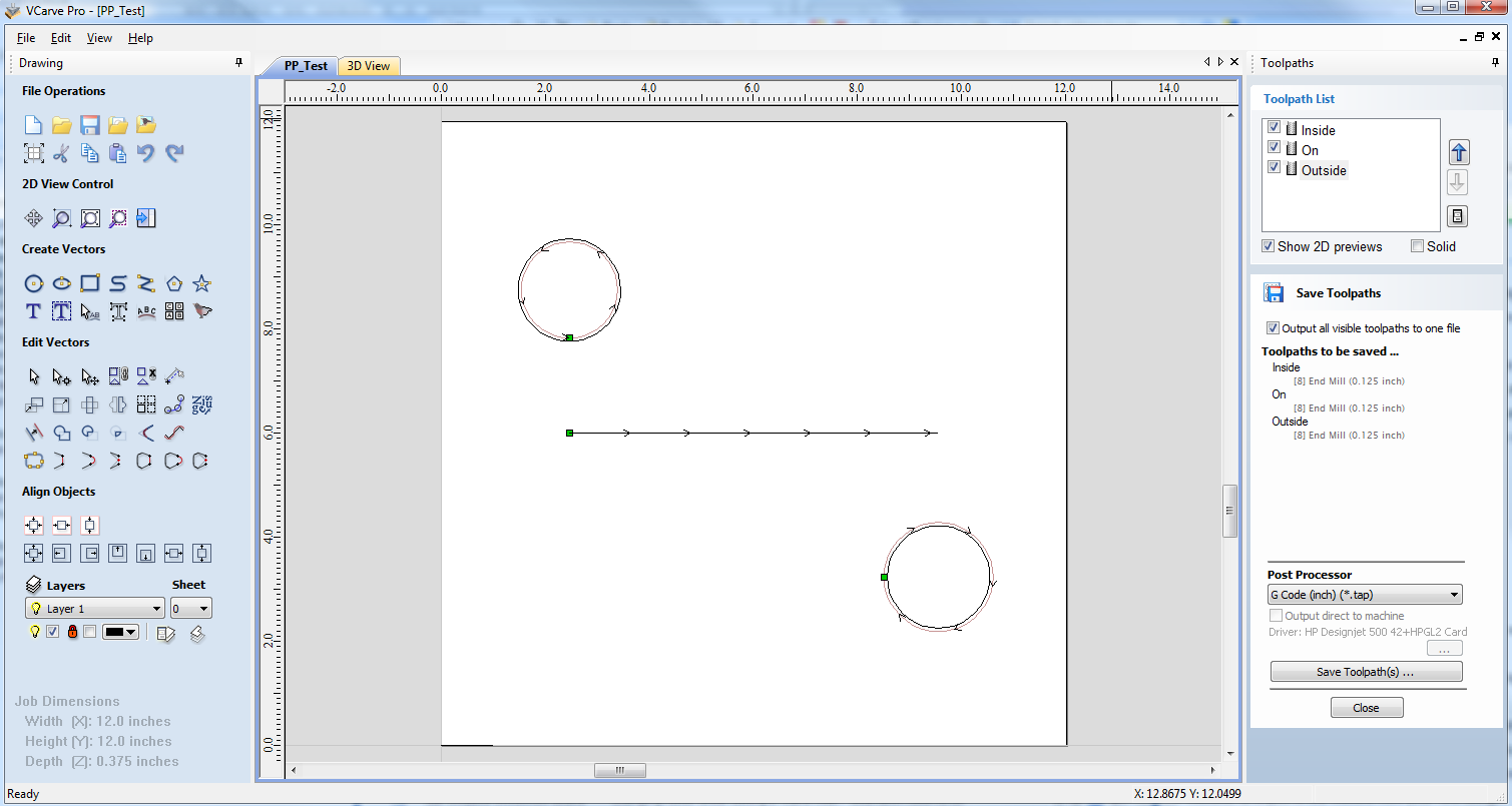
基本のポストプロセッサを使用して工具経路を保存し、任意のテキストエディタで内容を確認します。以下は、「G-Code Arcs (inch) (*.tap)」ポストプロセッサを使用してポストが行われたテストファイルの例です。以下の例では、Notepad ++エディタを使用して表示しています。
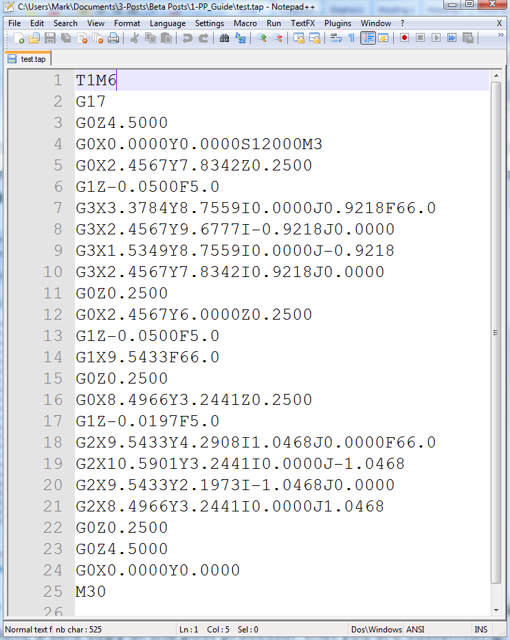
例えば、このポストプロセッサに工具変更セクションを加えていきます。まず、カスタイマイズを行うポストプロセッサのコピーを作成します。テキストエディタでポストプロセッサを開くと、テストファイルの出力をフォーマットしたポストプロセッサ内のテキスト行を確認することができます。
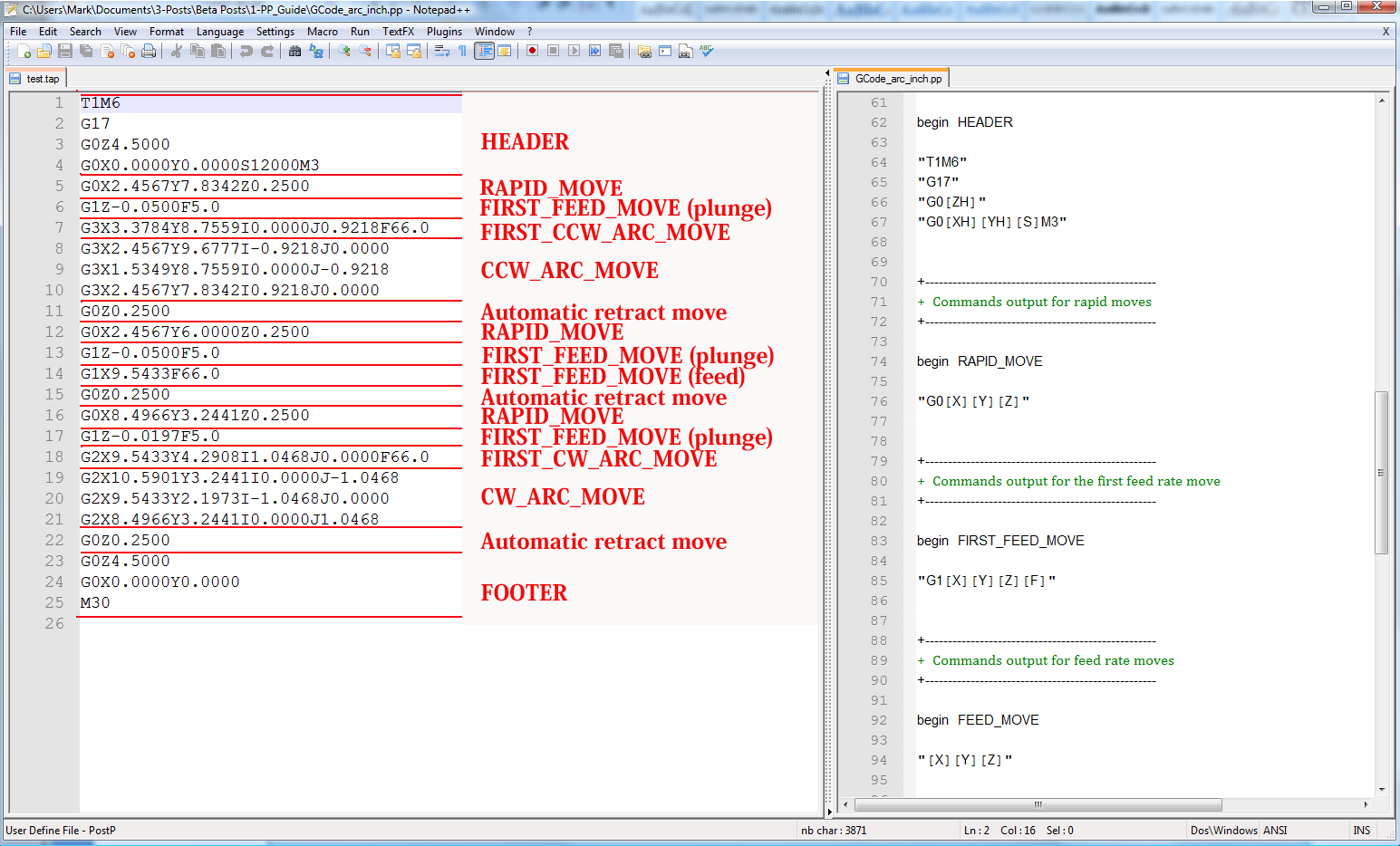
PostPフォルダは、アプリケーションのメインメニューから「ファイル > アプリケーションデータフォルダーを開く」を選択してアクセスします。
ポストプロセッサに工具変更セクションを追加するには、工作機械のコントロール(またはコントロールのソフトウェア)のドキュメントを参照する必要があります。たとえば、特定の工作機械に対して工具変更を実行するために追加する命令が、以下のようであると仮定します。
- M05命令は、工具変更前にスピンドルをオフにします。
- M0命令は、既存の工具を工具ホルダーに戻します。
- M06TTool_Number n命令は、工具番号nの新規工具を選択します。
- G43HTool_Number n命令は、コントロールに対し、工具番号nに工具長のオフセットを使用するように命令します。
- Sxxx M03は、回転速度をxxxに設定し、スピンドル(時計回りの回転)をオンにします。
任意のテキストエディタを使用してポストプロセッサを編集
使用するコンピューターのオペレーティングシステムがMicrosoft Vistaで、ユーザーアクセス制御が有効になっている場合、編集するポストプロセッサをPostPフォルダーからユーザー領域下のフォルダーにコピー、または移動します。
ファイル内で最初に編集すべきセクションは履歴コメントで、ここに変更内容を記載します。
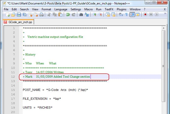
次に、当該ポストプロセッサ出力が、自動工具変更(ATC)コマンドを出力することを明示するように、POST_NAMEを編集します。これにより、新規のポストプロセッサは、ポストプロセッサのリストで「G-Code ATC Arcs (inch)(*.tap)」と表示されるようになります。
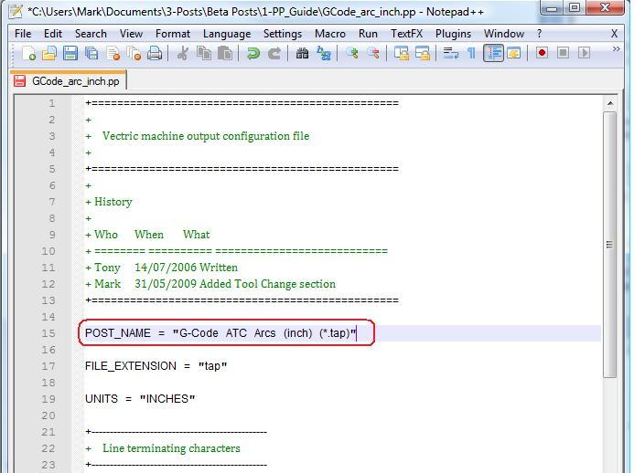
続いて、命令を含む工具変更セクションを追加します。ファイル内における新規セクションの場所は重要ではありませんが、ヘッダーと早送り動作セクションの間が、挿入に適しています。
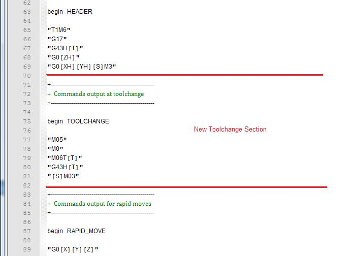
新規セクションの最初に、(「+」文字で始まる)コメント行を追加します。これにより、ファイル全体が読みやすくなります。ポストプロセッサに、各工具変更に対して以下の命令の出力を命令するために、「begin TOOLCHANGE」行を入力します(コマンドがヘッダーに含まれている最初の工具変更を除く)。
必要な命令を二重引用符で囲んで入力します。例の3行目と4行目にある“[T]”は、ファイルのポストプロセスが行われると工具番号で代用されます。5行目にある“[S]”は、工具の回転速度で代用されます。
最後に、ファイルに変更を保存します。すでにPOST_NAMEを変更してあるので、「GCODE_ATC_Arcs_inch.pp」のような新規名でファイルを保存します。
使用するコンピューターのオペレーティングシステムがMicrosoft Windows 7またはMicrosoft Vistaで、ユーザーアクセス制御が有効になっている場合、編集済みのファイルを「PostP」フォルダーにコピーして戻します。
ソフトウェアの実行中に新規のポストプロセッサをテストする場合は、ソフトウェアを再起動します。
ポストプロセッサに構文エラーがある場合、ソフトウェアの開始時に次図のようなエラーが表示されます。また、編集を行ったポストプロセッサは、ポストプロセッサ構成ファイルのドロップダウンリストに表示されません。すべてのエラーを修正し、ソフトウェアを再起動します。
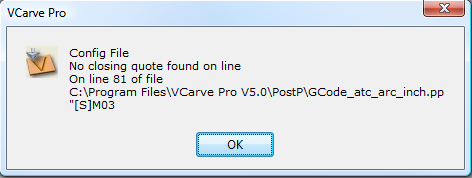
ソフトウェアの再起動時にエラーが表示されない場合、テストファイルを開き、単数または複数のテスト工具経路を保存します。
ポストプロセッサ構成ファイルのドロップダウンリストからポストプロセッサを選択し、「工具経路保存」ボタンをクリックします。
テキストエディタで保存したファイルを確認します。
ファイルの内容に問題がなければ、マシン上でファイルを試行します。
修正したポストプロセッサからの出力を初めて実行する場合は、細心の注意を払ってください。
例: ファイル拡張子の変更
ポストプロセッサに自動的に生成されたファイル拡張子は、「工具経路保存」ボタンのクリックにより表示される「名前を付けて保存」ダイアログ内で変更することができます。
しかし、 毎回ファイル拡張子を変更する代わりに、ポストプロセッサから生成されるファイル拡張子を永久に変更することもできます。
以下のように実行します。
編集するポストプロセッサのコピーを作成してください。
ポストプロセッサ構成ファイルは、「.PP」拡張子付きで、製品インストールフォルダーの「PostP」フォルダーに保存されています。Aspireバージョン2では、デフォルトのPostP folderは「C:\Program Files\Aspire V2.0\PostP」です。PostPフォルダーの場所は、インストールされた製品と、ソフトウェアのインストール時にソフトウェアがカスタムロケーションにインストールされたかにより異なります。
任意のテキストエディタを使用してポストプロセッサを編集します。
使用するコンピューターのオペレーティングシステムがMicrosoft Windows 7またはMicrosoft Vistaで、ユーザーアクセス制御が有効になっている場合、編集するポストプロセッサをPostPフォルダーからユーザー領域下のフォルダーにコピー、または移動します。
ポストプロセッサ構成ファイル内で、以下の2行で始まる行を検索します。
POST_NAME =
FILE_EXTENSION =
これらを変更します。
例えば、「G Code ATC (inch)(*.tap)」ポストプロセッサに生成されるファイル拡張子を「.tap」から「.nc」に変更します。その場合、
POST_NAME = "G Code ATC (inch) (*.tap)"
FILE_EXTENSION = "tap"
を以下のように編集します。
POST_NAME = "G Code ATC (inch) (*.nc)"
FILE_EXTENSION = "nc"
変更をファイルに保存します。使用するコンピューターのオペレーティングシステムがMicrosoft Windows 7またはMicrosoft Vistaで、ユーザーアクセス制御が有効になっている場合、編集済みのファイルを「PostP」フォルダーにコピーして戻します。
ソフトウェアの実行中に新規のポストプロセッサをテストする場合は、ソフトウェアを再起動します。ポストプロセッサに構文エラーがある場合、ソフトウェアの開始時に次図のようなエラーが表示されます。また、編集を行ったポストプロセッサは、ポストプロセッサ構成ファイルのドロップダウンリストに表示されません。すべてのエラーを修正し、ソフトウェアを再起動します。
ソフトウェアの再起動時にエラーが表示されない場合、テストファイルを開き、単数または複数のテスト工具経路を保存します。
ポストプロセッサ構成ファイルのドロップダウンリストからポストプロセッサを選択し、「工具経路保存」ボタンをクリックします。
テキストエディタで保存したファイルを確認します。
ファイルの内容に問題がなければ、マシン上でファイルを試行します。
修正したポストプロセッサからの出力を初めて実行する場合は、細心の注意を払ってください。
ヒント
- 最初からやり直す場合を考慮し、必ず編集を行うポストプロセッサのコピーを作成してください。
- ポストプロセッサの編集にMicrosoft Wordなどのワードプロセッサプログラムを使用する場合は、ファイルをテキスト形式で保存してください。
ファイルにフォーマット情報を含めることはできません。 - Microsoft Windows 7またはMicrosoft Vistaを実行するコンピューターでポストプロセッサを編集する場合は、「Program Files\Product folder\PostP」フォルダー内で直接ファイルの編集を行わないでください。常に、ユーザー領域内でファイルを編集し、編集済みのファイルを「Program Files\Product folder\PostP」にコピーしてください。
- 変更を加える場合は、「+」または「|」文字で開始するコメントを使用してください。
コメントはプログラムに作用しませんが、変更の記録により、将来変更を理解する際に役立ちます。 - 全ての命令を二重引用符で囲んでください。
- 可能な限り、行番号を利用できるテキストエディタを使用してください。ファイル内でエラーが検出され、ポストプロセッサのデバッグを行う際に有用です。プログラムの開始時に、プログラムはPostPフォルダー内のポストプロセッサをチェックします。ファイル内に構文エラーが存在する場合、最初に検出された行番号を示すエラーメッセージが表示されます。
- ポストプロセッサの編集が完了したら、必ずコピーを作成してください。より新しいバージョンのVectric製品をインストールする場合は、新バージョンのソフトウェアのPostPフォルダーに修正済みのポストプロセッサをコピーしてください。初めて工具経路を保存する際に、修正済みのポストプロセッサを選択してください(ソフトウェアは選択を記憶するため後続動作では不要)。
- 別バージョンのソフトウェアをインストール、またはソフトウェアのバージョンをアップグレードする場合は、新バージョンのPostPフォルダーに修正済みのポストプロセッサをコピーしてください。初めてファイルのポストプロセスを行う場合は、ソフトウェアの新バージョンが使用されるように、適切なポストプロセッサを選択してください。
- 新しいバージョン(V5.5以降)のソフトウェアでは、アプリケーションで「ファイル > アプリケーションデータフォルダーを開く...\PostP」をクリックして、ポストプロセッサにアクセスすることができます。
- ポストプロセッサのカスタマイズリストは、「ファイル > アプリケーションデータフォルダーを開く...\My_PostP」に必要なポストプロセッサのみをコピーして作成することができます。.ppファイル拡張子を持つファイルが「My_PostP」フォルダーに存在する場合、「My_PostP」フォルダーに存在するポストプロセッサのみが、ポストプロセッサのドロップダウンリストに表示されます。