User Guide
- 2D Design and Management
- Interface Overview
- 2D Design and Management
- 3D Design and Management
- 3D Toolpath Files
- Rotary Machining and Wrapping
- Creating a Rotary Job
- Importing External Models in a Rotary Project
- Simple Rotary Modelling using 2D Toolpaths
- Modelling 3D Rotary Projects
- Advanced Modelling of 3D Rotary Projects
- Postprozessor-Bearbeitung
2D Design and Management
The 2D View is used to design and manage the layout of your finished part. Different entities are used to allow the user to control items that are either strictly 2D or are 2D representations of objects in the 3D View. A list of these 2D View entities are described briefly below and more fully in later sections of this manual.
Ultimately the point of all these different types of objects is to allow you to create the toolpaths you need to cut the part you want on your CNC. This may mean that they help you to create the basis for the 3D model or that they are more directly related to the toolpath such as describing its boundary shape. The different applications and uses for these 2D items mean that organization of them is very important. For this reason Aspire has a Layer function for managing 2D data. The Layers are a way of associating different 2D entities together to allow the user to manage them more effectively. Layers will be described in detail later in the relevant section of this manual. If you are working with a 2 Sided project you can switch between the 'Top' and 'Bottom' sides in the same session, enabling you to create and edit data on each side, and using the 'Multi Sided View' option you can view the vectors on the opposite side. 2 Sided Setup will be described in detail later in the relevant section of this manual.
 Vectors
Vectors are lines, arcs and curves which can be as simple as a straight line or can make up complex 2D designs. They have many uses in Aspire, such as describing a shape for a toolpath to follow or creating designs. Aspire contains a number of vector creation and editing tools which are covered in this manual.
As well as creating vectors within the software many users will also import vectors from other design software such as Corel Draw or AutoCAD. Aspire supports the following vector formats for import: *.dxf, *.eps, *.ai, *.pdf, *skp and *svg. Once imported, the data can be edited and combined using the Vector Editing tools within the software.
Bitmaps
Although bitmap is a standard computer term for a pixel based image (such as a photo) in *.bmp, *.jpg, *.gif, *.tif, *.png and *.jpeg. These file types are images made up of tiny squares (pixels) which represent a scanned picture, digital photo or perhaps an image taken from the internet.
To make 3D models simple to create, Aspire uses a method which lets the user break the design down into manageable pieces called Components. In the 2D View a Component is shown as a Grayscale shape, this can be selected and edited to move its position, change its size etc. Working with the Grayscale's will be covered in detail later in this manual. As with bitmaps, many of the vector editing tools will also work on a selected Component Grayscale.
Interface Overview
- The Main Menu Bar (the Drop Down Menus) along the top of the screen (File, Edit, Model, Toolpaths, View, Gadgets, Help) provides access to most of the commands available in the software, grouped by function. Click on any of the choices to show a Drop-Down list of the available commands.
- The Design Panel is on the left side of the screen. This is where the design tabs can be accessed and the icons within the tabs to create a design.
- The Toolpath Tab is on the right side of the screen. The Top section of the toolpaths tab houses all of the icons to create, edit and preview toolpaths. The bottom half shows you toolpaths that you have already created.
- The 2D Design window is where the design is drawn, edited and selected ready for machining. Designs can be imported or created directly in the software. This occupies the same area as the 3D View and the display can be toggled between the two using F2 and F3 or the tabs at the top of the window.
- The 3D View is where the composite model, toolpaths and the toolpath preview are displayed.
- If you wish to see the 2D and 3D views simultaneously, or you wish to switch your focus to the Toolpaths tab at a later stage of your design process, you can use the interface layout buttons (accessible in the 2D View Control section on the Drawing Tab) to toggle between the different preset interface layouts.
Managing the Interface
The tool pages have Auto-Hide / Show behavior which allows them to automatically close when not being used, thus maximizing your working screen area.
The software includes two default layouts, one for designing and one for machining, which can automatically and conveniently set the appropriate auto-hide behavior for each of the tools pages. Toggle layout buttons on each of the tools pages allow you to switch the interface as your focus naturally shifts from the design stage to the toolpathing stage of your project.
Accessing Auto-hidden tabs
If a tools page is auto-hidden (because it is currently unpinned, see pinning and unpinning tools pages, below), then it will only appear as a tab at the side of your screen. Move your mouse over these tabs to show the page temporarily. Once you have selected a tool from the page, it will automatically hide itself again.
Pinning and unpinning tools pages
The auto-hide behavior of each tools page can be controlled using the push-pin icons at the top right of the title area of each page.
Default layout for Design and Toolpaths
Aspire has two default tool page layouts that are designed to assist the usual workflow of design, followed by toolpath creation.
In all three of the tools tabs there are 'Switch Layout' buttons. In the Drawing and Modeling tabs, these buttons will shift the interface's focus to toolpath tasks by 'pinning-out' the Toolpaths tools tab, and 'unpinning' the Drawing and Modeling tools tabs. In the toolpaths tab, the button reverses the layout - unpinning the toolpaths page, and pinning-out the Drawing and Modeling pages.You can toggle between these two modes using the F11 and F12 shortcut keys.
2D Design and Management
The 2D View is used to design and manage the layout of your finished part. Different entities are used to allow the user to control items that are either strictly 2D or are 2D representations of objects in the 3D View. A list of these 2D View entities are described briefly below and more fully in later sections of this manual.
Ultimately the point of all these different types of objects is to allow you to create the toolpaths you need to cut the part you want on your CNC. This may mean that they help you to create the basis for the 3D model or that they are more directly related to the toolpath such as describing its boundary shape. The different applications and uses for these 2D items mean that organization of them is very important. For this reason Aspire has a Layer function for managing 2D data. The Layers are a way of associating different 2D entities together to allow the user to manage them more effectively. Layers will be described in detail later in the relevant section of this manual. If you are working with a 2 Sided project you can switch between the 'Top' and 'Bottom' sides in the same session, enabling you to create and edit data on each side, and using the 'Multi Sided View' option you can view the vectors on the opposite side. 2 Sided Setup will be described in detail later in the relevant section of this manual.
Vectors
Vectors are lines, arcs and curves which can be as simple as a straight line or can make up complex 2D designs. They have many uses in Aspire, such as describing a shape for a toolpath to follow or creating designs. Aspire contains a number of vector creation and editing tools which are covered in this manual.
As well as creating vectors within the software many users will also import vectors from other design software such as Corel Draw or AutoCAD. Aspire supports the following vector formats for import: *.dxf, *.eps, *.ai, *.pdf, *skp and *svg. Once imported, the data can be edited and combined using the Vector Editing tools within the software.
Bitmaps
Although bitmap is a standard computer term for a pixel based image (such as a photo) in *.bmp, *.jpg, *.gif, *.tif, *.png and *.jpeg. These file types are images made up of tiny squares (pixels) which represent a scanned picture, digital photo or perhaps an image taken from the internet.
To make 3D models simple to create, Aspire uses a method which lets the user break the design down into manageable pieces called Components. In the 2D View a Component is shown as a Grayscale shape, this can be selected and edited to move its position, change its size etc. Working with the Grayscale's will be covered in detail later in this manual. As with bitmaps, many of the vector editing tools will also work on a selected Component Grayscale.
3D Design and Management
As well as creating toolpaths directly from 2D drawings, Aspire can produce extremely flexible 3D toolpaths. These toolpaths are created from 3D design elements called 3D Components that can be generated from models created in external 3D design packages, imported as 3D clipart or built entirely from within Aspire using 2D artwork as a source.
The 3D View
The 3D View can show you the current Composite Model (which is built from all of the currently visible 3D Components and Levels), the Toolpath Preview (a highly accurate 3D simulation of the resulting physical object that will result from your toolpaths called the Preview Material Block). Which of these is currently displayed will depend on whether or not you have a part which has 3D Components and Toolpaths or are just working on something that only includes 2D Data.
Whenever you have the Preview Toolpaths form open on the Toolpaths tab, the 3D View displays the Preview Material Block instead of the Composite Model. When this is closed if you are working on a part that only includes 2D data and 2D or 2.5D toolpaths it will continue to display the Preview Material Block. If your part contains any visible 3D Components then as soon as the Preview Toolpaths form is closed it will revert to showing the Composite Model in the 3D View and hide the simulation. In addition to these items, you can see line drawings of any calculated toolpaths in the 3D View. The visibility of these calculated toolpaths can be controlled from the Toolpath List on the Toolpaths tab using the check-boxes next to the toolpaths name. If working in a 2 Sided environment you can view both sides of a project in the 3D View using the Multi Sided View option.
The Composite Model
Aspire has been designed to work in a way which enables the user to easily create even very complex projects. In any situation, the best approach to producing something complicated is to break it down into smaller pieces until a level of simplicity is reached that can be understood and managed. In Aspire this is achieved by letting the user work with pieces of the design which are combined to make the finished part. In the terminology of the software these pieces are called Components. To help organize the Components they are assigned to Levels. Step by step, Components and Levels can be created and modified until you have all the elements you need. In the images below you can see an example of how this might work. On the left you can see the separate component for a model of a bunch of grapes and on the right you can see these positioned to make the complete part - we call this resulting combination the Composite Model.
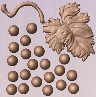
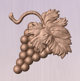
There is no limit to how simple or complex a Component or the Components on a Level can be (this is the user's choice). In the example shown, you can see that a model of a whole bunch of grapes may be made up of smaller individual components but they could also be combined to exist as one single Component (the assembled bunch of grapes) that could then be used to lay-out a more complex part with multiple bunches of grapes. They could also be organized so all the grapes were on one Level and leaf and stem on another to provide a different way of managing and manipulating the shapes. Each user will find a level of using Components and Levels they are comfortable with which may be dependent on the particular job or level of proficiency with the modeling tools.
3D Components and Levels
In Aspire, the aim is to end up with a set of Components and Levels that when combined together will make the finished 3D part. One way to think of this is like building a 3D collage or assembly. As the design evolves, new Levels or shapes may need to be created or existing ones changed. The parts of the collage are managed with the Component Tree which will be covered in more detail later.
Creating and Editing Components
An existing Component can be copied, scaled and have other edits carried out on it as an object. The user can also change the way it relates to the other Components, for instance whether it sits on top or blends into an overlapping area of another Component. The shape, location and relation of these pieces determine the look of the final part. As the job progresses, the user will need to create brand new Components or edit existing ones by adding new shapes, combining them with others or sculpting them.
Components can be created and edited by:
- Use a modelling tool to create shapes from 2D vectors.
- Import a pre-created 3D model - either a model previously created in Aspire or from another source such as a clipart library or a different modelling package.
- Create a 'texture' Component from a bitmap image.
- Use the Split Components Tool to break an existing Component into multiple pieces.
All of these methods are covered in detail throughout the training material.
Dynamic Properties
As well as having its underlying 3D shape, each component also has a number of dynamic properties that can be freely modified without permanently changing its true shape. These include scaling of the Component's height, the ability to tilt it, or to apply a graduated fade across it.
These dynamic properties can always be reset or altered at any time during your modeling process, which makes them a particularly useful way of 'tweaking 'your components as you combine them together to form your final composite model.
Combine Modes
The Combine Mode is a very important concept when working with 3D shapes within Aspire. The options for combine mode are presented when creating new shapes and also when deciding how Components and Levels will interact in the Component List. Rather than cover this in every section where it is applicable, it is worth summarizing the options here so the general concept can be understood.
When you have more than one 3D shape, such as the Component pieces of the design or where you have an existing shape and are creating a new one, then you need to have a way to tell the software how the additional entities will interact with the first. This can be an abstract concept for users who are new to 3D but it is an important one to grasp as early as possible. In Aspire this is controlled by a choice called the Combine Mode.
There are four options for this: Add, Subtract, Merge High, Merge Low.
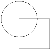
As modeling is an artistic and creative process, there is no general rule to describe when to use each one. As a guide though you can assume that if the second shape's area is completely within the originals one then you will probably be adding or subtracting and if the shapes only partly overlap that you will probably use Merge or, very occasionally, Low.
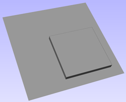
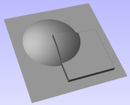
The four options and their specific effects are described on the following pages. To illustrate the different effects a combination of an overlapping beveled square and a dome will be used. You can see in the image top right how these are arranged in the 2D View and how they overlap. Then you can see each individual shape in the images below middle and right. These shapes will be used to demonstrate the different Combine Modes. In every case the Dome will be considered the primary shape and the square is the secondary shape which is being combined with the first. In addition to the dome/square example some images of 'real world' parts will also be included to help to understand how these can be used on actual projects.
As well as working on individual shapes, the Combine Modes are also assigned to Levels. These will govern how the combination of all the individual components on one Level interacts with the result of all the Components on the Level below it in the Component Tree
Note:
There is a 5th Combine Mode available from the right mouse click menu after a component has been created called Multiply. This combine mode has specialist applications which are dealt with in the appropriate tutorial videos. This option will literally multiply the heights of the Component or Levels being combined to create the new Composite 3D shape.
Add
When Add is selected, it takes the first shape and then just adds the height of the second shape directly on top of the first. Any areas which overlap will create a shape which is exactly the height of each shape at that point added together (see below)
Typically the add option is mainly used when the shape being added sits completely within the original shape, this ensures that the uneven transition where the parts only partly overlap (as shown in the example) do not occur.
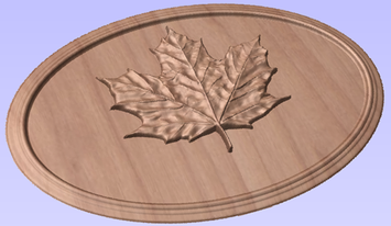
The example above shows the Maple Leaf and border extrusion Components being Added to the dome Component in the sign example from the Introduction to Modeling document.
Subtract
When Subtract is selected it takes the first shape and then removes the height of the second shape from the first. Any areas which overlap will be a combination of the original height/shape less the second shape. Areas where the shape goes into the background will become negative regions. You can see how this looks using the dome and square in the image below:
Typically subtract, like the add option, is mainly used when the shape being removed sits completely within the original shape, this ensures that the uneven transition where the parts only partly overlap (as shown in the example) do not occur.
The image shown above has some 'creases' to help define the muscles of the lioness. The shapes to create these recesses were created by using the Subtract option with the Create Shape tool on the vectors representing those recessed areas.
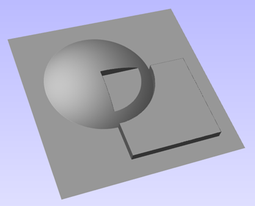
Merge
When the Merge option is selected any areas of the shapes which do not overlap remain the same. The areas that overlap will blend into each other so that the highest areas of each are left visible. This results in the look of one shape merging into the other and is in effect a Boolean union operation. You can see how this looks using the dome and square in the image below:
Typically the merge option is used when the shape being combined partly overlaps the original shape. This enables a reasonable transition to be made between them.
The image above shows 2 Herons, a rope border and banner Components. Each of these overlaps with the others and so they are set to Merge in this areas. Whatever is the higher of the two merged areas is what is prominent. In this case the rope is lower than everything and the Banner is higher than the Herons so the desired effect can be achieved.
Low
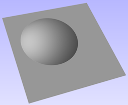
The Low option is only available when combining Components (not in the modeling tools). When this mode is selected, any areas which do not overlap are left as they were in the original two shapes. Any areas which overlap will create a new shape which is the lowest points taken from each shape, this is in effect a Boolean intersection operation. You can see how this looks using the dome and square in the image below:
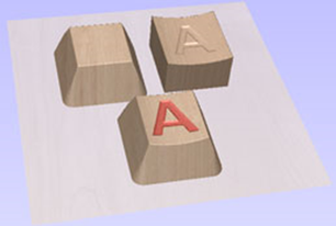
The Low option is used for recessing a shape into a raised shape. An example of this is shown in the image above.
The example shown on the right above uses the Low option to combine the flat topped 'button' component on the left with the curved top face component with the letter 'A' on the right. Combining both components with the merge low option gives the keyboard button with the curved top you see in the bottom row.
Level Mirror Modes
Right-clicking Levels in the component tree will open a pop-up menu offering commands and operations related to the clicked level and Mirror Modes can be set in this way. If a mirror mode is set on a Level, all the components it contains will be continually mirrored dynamically as they are moved, transformed or edited. The mirroring is non-destructive, that is it can be turned off or on at any time and does not alter the underlying components in any permanent way. Working inside a Mirror modes Level is a simple way of achieving a complicated symmetrical pattern by editing only one half (or quarter, see below) of the design.
The available Mirror Modes are broadly divided into two groups. The first group apply one plane of symmetry:
- Left to Right
- Right to Left
- Top to Bottom
- Bottom to Top

These modes allow you to work in one half of your job and the other half will be automatically and dynamically generated for you. For example, in Left to Right mode you would place your components in the left half of your job and a mirrored equivalent of each would be created in the other half of the job. This 'reflection' is updated dynamically as you work.
The other group offer two planes of symmetry (horizontal and vertical):
- Top Left Quadrant
- Top Right Quadrant
- Bottom Left Quadrant
- Bottom Right Quadrant
When using these modes your components should all be in the quadrant (quarter) of the job. Mirrored reflections horizontally and vertically will be created in the other quadrants of the job for you.
Multi Sided View

When working in a 2 Sided environment you can create components independently per side or using the Right click option you can copy or move a component to the opposite side. Selecting the option to work in 'Multi Sided View' allows you to view components you may have on the Top and Bottom side in the 3D View. In the Toolpath Preview form of a project that contains toolpaths for the Top and Bottom Sides the multi sided view presents the simulation of the toolpath preview on both sides also, if the multi sided view is not selected you can use the 'Preview all Sides' option in the Toolpath Preview form to display the Top and Bottom Toolpaths in the 3D view. 2 Sided Setup will be described in detail later in the relevant section of this manual.
3D Toolpath Files
Files from Vectric's Cut3D, PhotoVCarve and Design and Make Machinist that include 3D toolpaths can be imported into Aspire using the main menu command: File ► Import ► PhotoVCarve, Machinist or Cut3D Toolpaths.
The 3D file must first be scaled to the required size before toolpaths are calculated, and then the complete file saved ready for importing into Aspire. These files can only be moved and positioned inside Aspire but cannot be scaled.
A Grayscale thumbnail of the 3D job is drawn in the 2D View with the X0 Y0 origin at the position it was set in Cut3D, PhotoVCarve or Design and Make Machinist. The associated toolpath(s) are also drawn in the 3D window and the names appear in the Toolpath list.
Positioning
To move the 3D design toolpaths open the 2D Window, click the Left mouse Twice on grayscale image (turns light Blue to indicate it's selected), then drag to the required position, or use the Move or Alignment tools for accurate positioning.
The toolpath(s) are automatically moved in the 3D window to the same XY position as the image.
Toolpaths for the example above have been calculated with the X0 Y0 in the middle of the 3D design. When imported into Cut2D the data is automatically positioned using the same coordinates, which places three quarters of the design off the job. In the second image the grayscale image has been moved to the middle of the job.
The 2D mirror and rotate drawing tools can also be used to edit the 3D data set.
3D toolpaths can also be copied using the Duplicate Toolpath command on the Toolpaths Tab making it very easy to use multiple elements from a single design on a job. The thumbnail preview is also copied for each toolpath, making it very easy to position additional copies of a 3D toolpath.
For example, a single design can be copied and mirrored to create Left and Right versions of a 3D design or to place multiple copies of a decorative design in the corners of a cabinet door panel as shown below.
Toolpaths for the 3D elements can be previewed along with the conventional Profile, Pocketing and Drilling toolpaths, and everything will be saved ready for machining.
A good example of where this functionality might be used in conjunction with PhotoVCarve is for making personalized picture frames that include the PhotoVCarve grooves plus descriptive engraved text and a decorative Profiled or Beveled border. As shown below:


Options
Imported toolpaths can also be edited to position them inside the material or to change the cutting parameters - speeds and feed rates can be changed.
Design and Make Machinist
When using a Design and Make Machinist file that includes multiple toolpaths, you must remember to edit the Start Depth for all of the imported 3D toolpaths.
Click the Edit toolpath icon or Double click on the toolpath name to open the edit form.
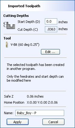
For example, after machining a half-inch deep pocket a PhotoVCarve design can then be edited to have a Start Depth = 0.5 inches and this will carve the photograph onto the base of the pocket surface.
Rotary Machining and Wrapping
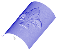
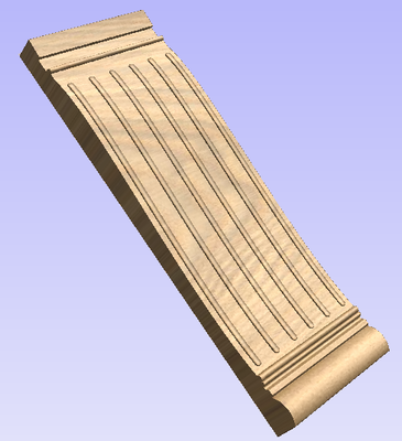
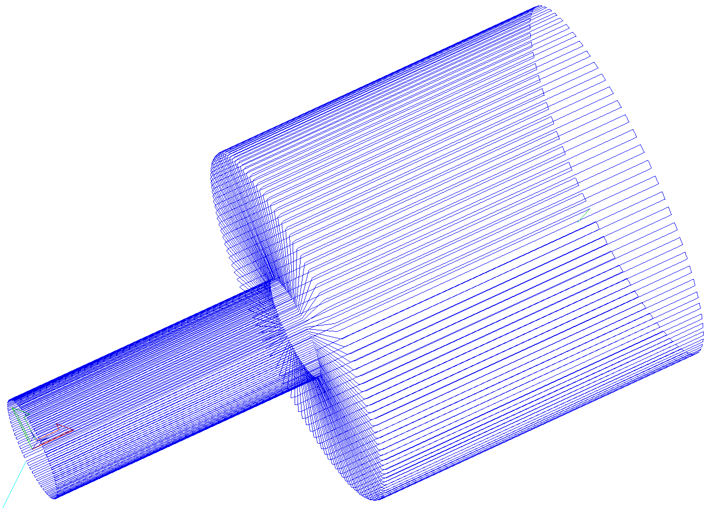
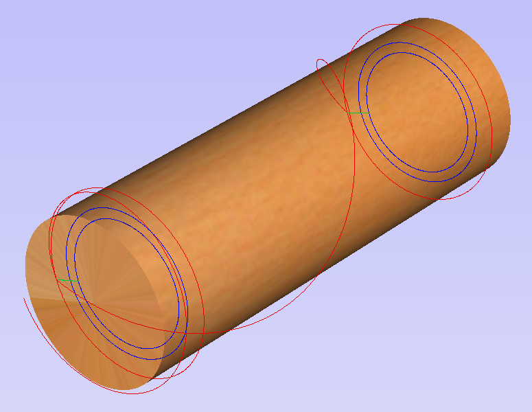
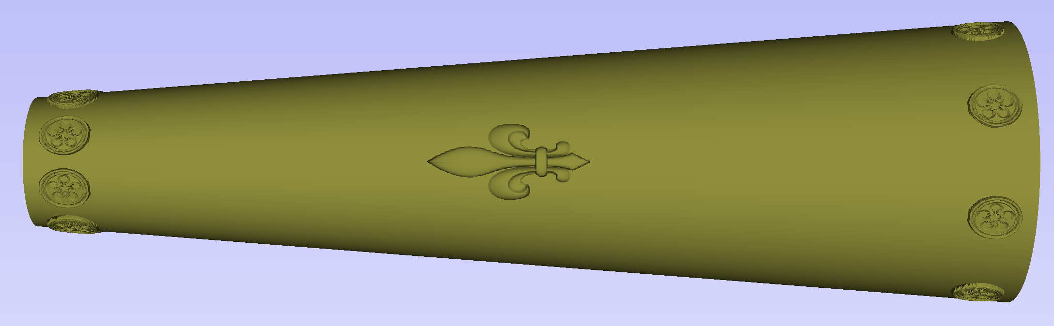
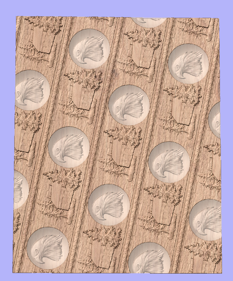
Aspire can 'wrap' flat toolpaths around a cylinder to provide output to CNC machines which are configured with a rotary axis / indexer. The image below shows a flat toolpath wrapped around part of a cylinder.
Note
It is important to note that wrapping works in conjunction with specially configured post-processors which take the XYZ 'flat' toolpaths and wrap them around a rotary axis, replacing either the X or Y moves with angular moves.
The toolpaths can be visualized wrapped within the program when the Auto Wrapping mode is on.
Aspire can also visualize a wrapped model within the program by drawing the shaded composite model wrapped.
Aspire also has the ability to draw the toolpath simulation wrapped. Although this is very useful for getting a feel for how the finished product will look, it is important to realize that the wrapped simulation may not be a 100% accurate representation of how the finished product will look. An example of potential difference would be if you drilled holes in your rotary job. In the actual work piece these will obviously just be round holes, in the wrapped simulation these may appear as distorted ovals due to the 'stretching' process which takes place when we wrap the flat simulation model for display.
Note
If your rotary axis is aligned along your Y axis you would choose the Orientation Along Y Axis option during job setup. All the examples in this document will assume that the rotary axis is aligned along X.
It is important to realize that there are a huge number of possible combinations of machine controller and axis orientations for rotary axis / indexers. This means it is impractical for Vectric to supply a pre-configured post-processor for every possible combination as standard. We include some wrapping post-processors in the software that can be configured when you setup your Machine Configuration.
If you need to select a new post, you can do so by accessing the Save Toolpaths menu. To do so, click the 'Manage machine configuration' button as seen in the image below:
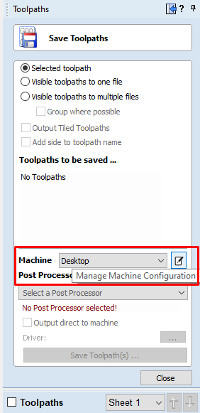
This will now open a menu where you can press the button under 'Associated Post-Processors' to access all of the available post-processors within the software and choose the appropriate wrapped post-processor for your machine configuration.
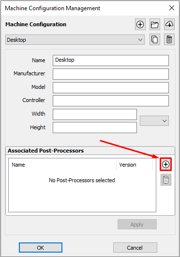
You can also right click the post in this menu and select 'view' to view the contents of the post, should you need to edit it later.
Examining these posts may be helpful if you need to configure a post of your own. If Vectric have not supplied a standard a post for your machine configuration please refer to the Post Processor Editing Guide accessible from the Help menu of the program for information on how to configure a post-processor and also look at the standard rotary posts Vectric supply.
You should also look at the Vectric forum to see if anyone else has already configured a post for your configuration or one similar. If, after looking at these resources you are still unsure of what needs to be done for your machine, please feel free to contact support@vectric.com for help. However, please note that we cannot guarantee to write a custom rotary post-processor for every individual requirement.
Creating a Rotary Job
Z Origin
You have the choice of specifying if the tool is being zeroed on the center of the cylinder or the surface. When you are rounding a blank, you cannot set the Z on the surface of the cylinder, as the surface it is referring to is the surface of the finished blank. We would strongly recommend for consistency and accuracy that you always choose 'Center of Cylinder' when outputting wrapped toolpaths as this should always remain constant irrespective of irregularities in the diameter of the piece you are machining or errors in getting your blank centered in your chuck.
Tip:
A useful tip for doing this is to accurately measure the distance between the center of your chuck and a convenient point such as the top of the chuck or part of your rotary axis mounting bracket. Write down this z-offset somewhere, and zero future tools at this point and enter your z-offset to get the position of the rotary axis center. Another reason for choosing 'Center of Cylinder' is that some controls will be able to work out the correct rotation speed for the rotary axis based on the distance from the center of rotation. If the Z value is relative to the surface, the control would need to know the diameter or radius of the cylinder at Z zero.
XY Origin
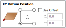
XY Drawing Origin - Here you can specify where the XY zero origin will be placed on your job. These options correspond to the same fields on the normal 'Job Setup' form within the program. Most people would use the default Bottom Left Corner, but for some jobs you may prefer to have the XY origin in the Center.
- In a job with horizontal orientation (Along X Axis), the X offset will correspond to the length of the cylinder, and the Y offset will be a point along its circumference.
- In a job with vertical orientation (Along Y Axis), it's the opposite. The Y offset will correspond to the length of the cylinder, and the X offset will be a point along its circumference.
Orientation
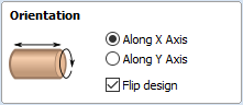
Cylinder Orientation Along - This section is used to tell the program how you have your rotary axis aligned on your machine. If you've already made your design, but just want to change the job for a different machine, then you could flip your design with the material so that all the vectors and components stay the same relative to the job.
Z Origin On - This section determines whether the Z Origin is set to the surface of the material or the base (center of cylinder). These settings can be over-ridden when the toolpath is actually saved, but we would strongly recommend the 'Cylinder Axis' is selected for rotary machining. The reasons for this are detailed in the note below.
Vector Layout
As well as creating a job at a suitable size for wrapping toolpaths, when creating the job, it will create a number of vectors which can be very useful when creating your wrapped job.
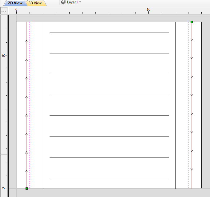
The vectors are created on their own individual layers and by default these layers are switched off to avoid cluttering up your work area. To switch on the layers, display the 'Layer Control' dialog (Ctrl+ L is the shortcut to show / hide this). To show / hide the layer simply click on the check box next to the layer name.
2Rail Sweep Rails - This layer contains two straight line vectors which can be used to sweep a profile along if you are creating a shaped column.
Bounding Box - This layer contains a rectangular vector covering the entire job area. This vector is useful if you are going to machine the complete surface of the cylinder.
Choosing stock material
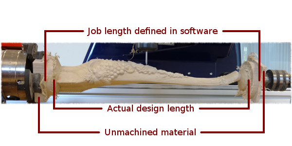
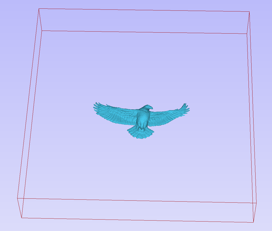
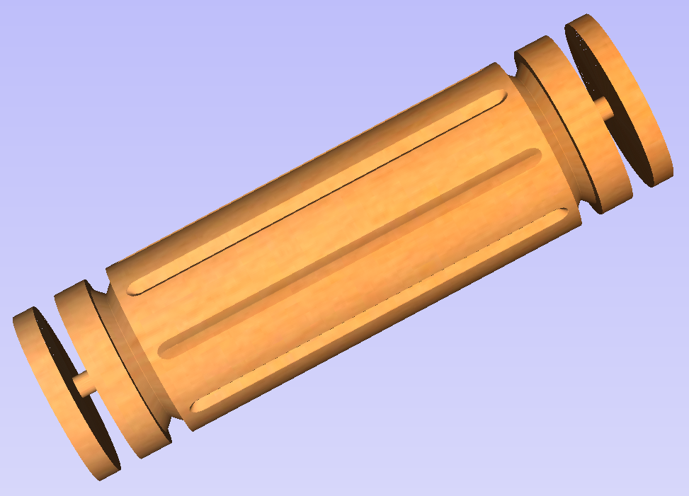
When setting-up rotary project, software assumes a perfect cylinder with an exact diameter. In practice the stock material may be uneven, or only blank with square profile may be available. In those cases blank needs to be machined into cylinder of desired size, before running toolpaths associated with the actual design.
Another consideration is length of the stock material. Typically, part of the blank will be placed within the chuck. It is also important that during machining, the cutting tool is always in safe distance from both chuck and tailstock. For those reasons, the blank has to be longer than the actual design. When setting-up the machine for cutting, one has to pay extra attention to ensure that origin is set accordingly to avoid the tool running into chuck or tailstock!
If the design was created without those considerations in mind, the blank size can always be adjusted in the Job Setup form.
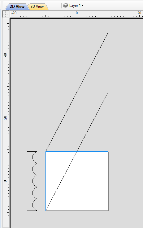
The picture below presents an example of a rotary project layout. As explained above, the actual blank is longer than job defined in Aspire to allow for the chuck and sufficient gaps. The actual design is shorter than job defined in Aspire, to leave some space for tabs, that can be machined with the profile toolpath prior to removing the finished part from the chuck.
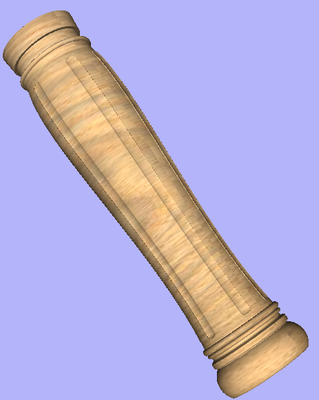
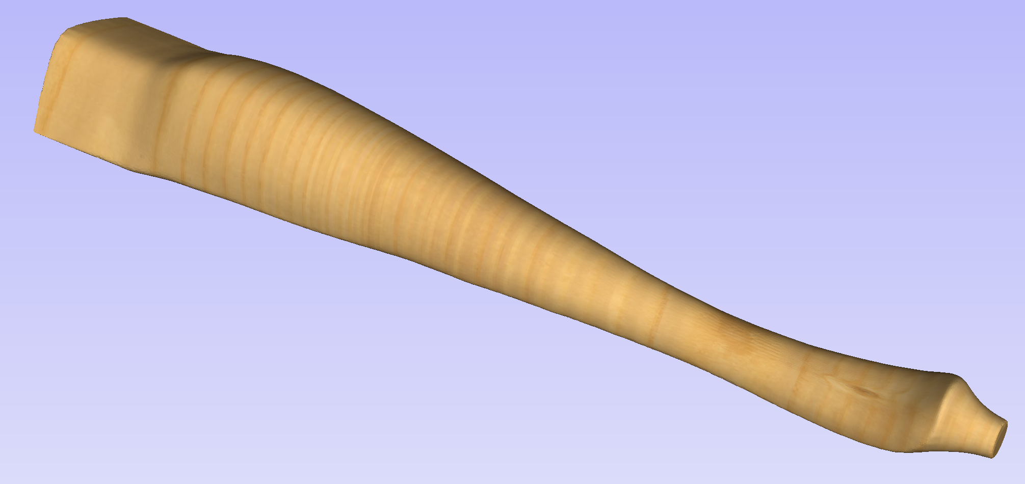
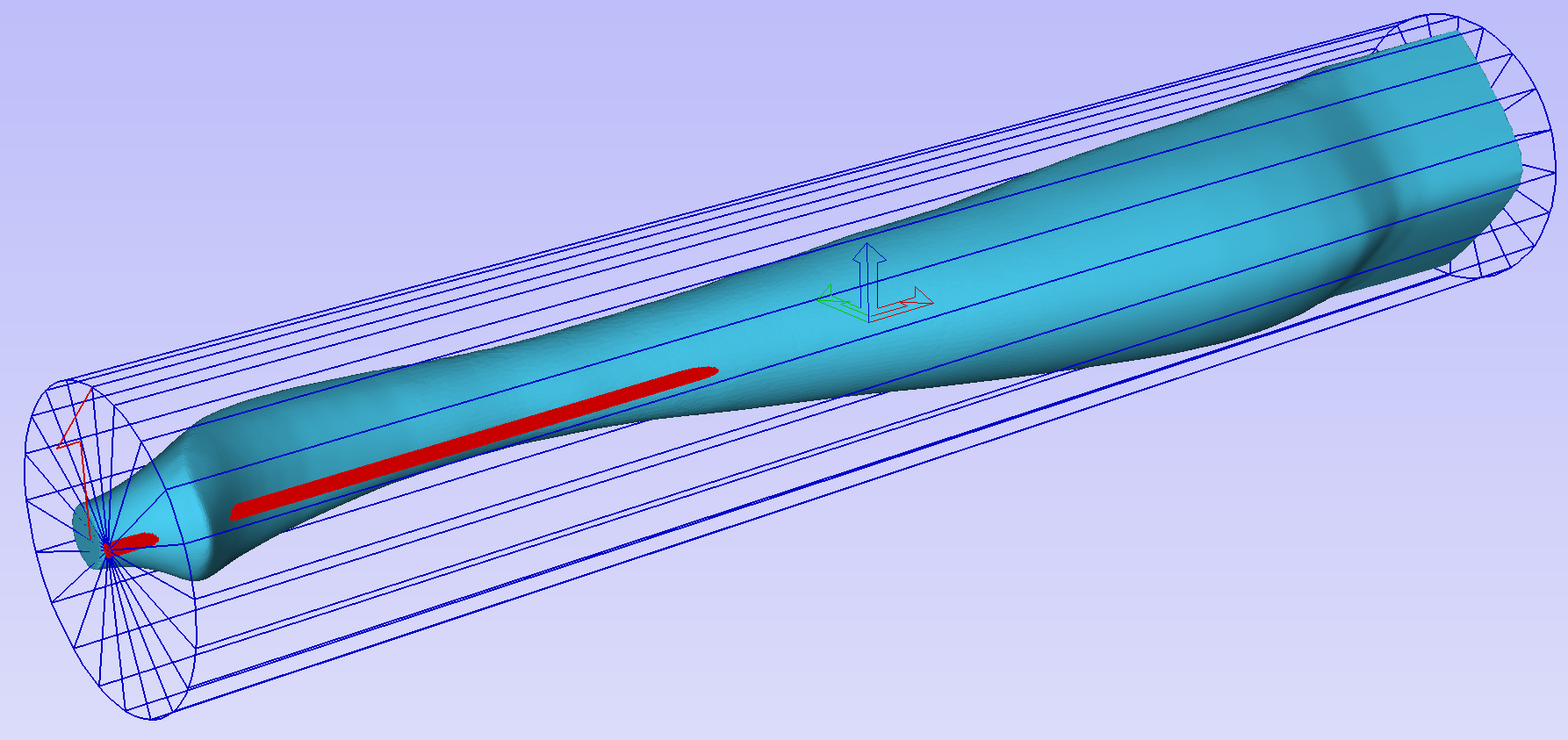
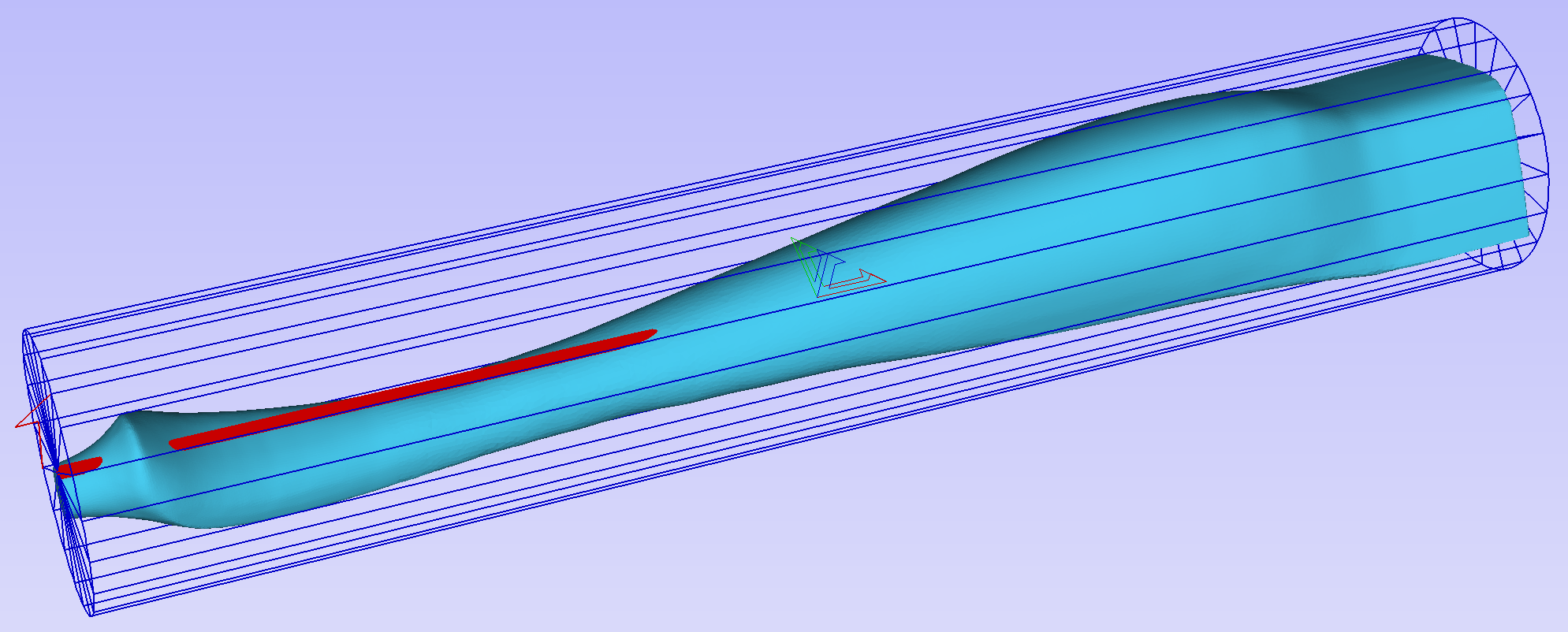
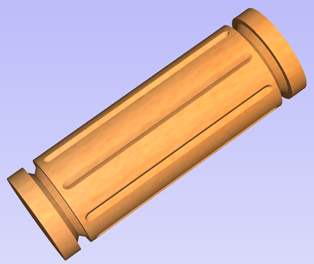
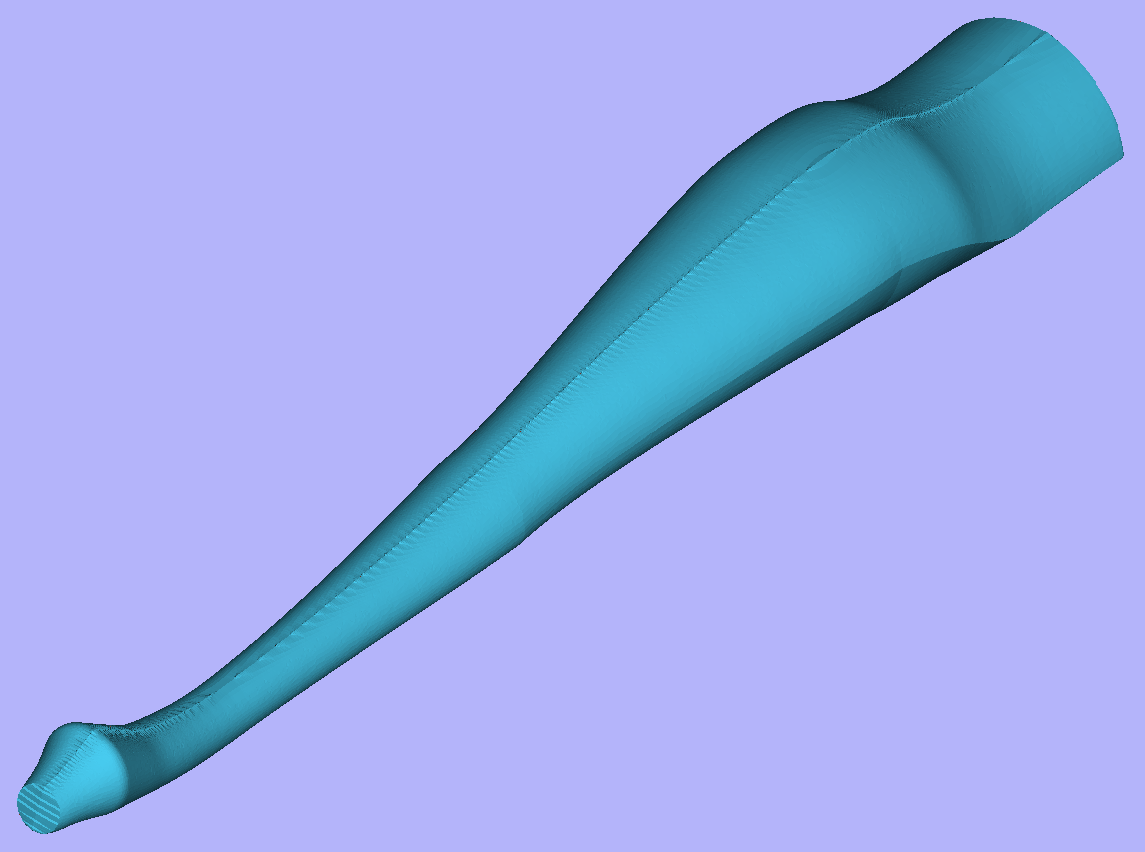
When machining 3D shapes with varying thicknesses like on the example shown below, it is a good idea to place the thicker end of the model on the side closest to the driving motor. This way torsional twisting will mostly affect the stronger end of the machined part and help to avoid bending or breaking of the part during machining.
Importing External Models in a Rotary Project
Importing Full-3D models
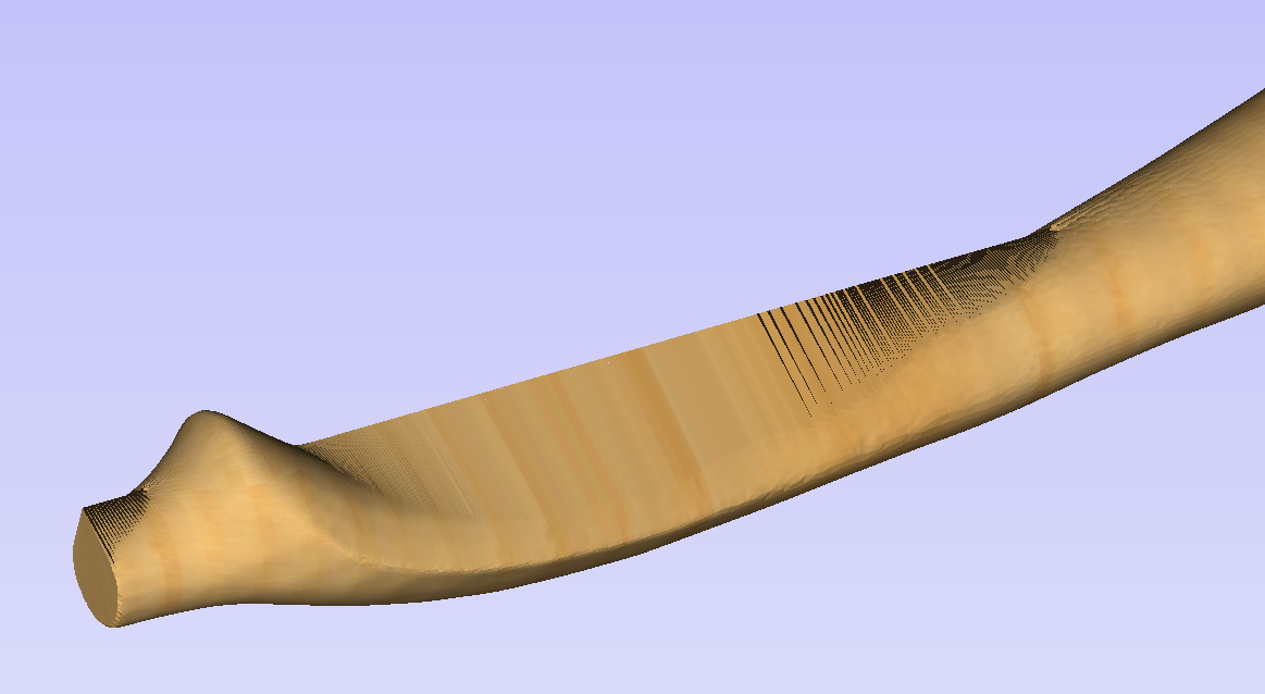
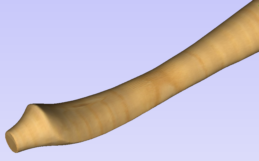
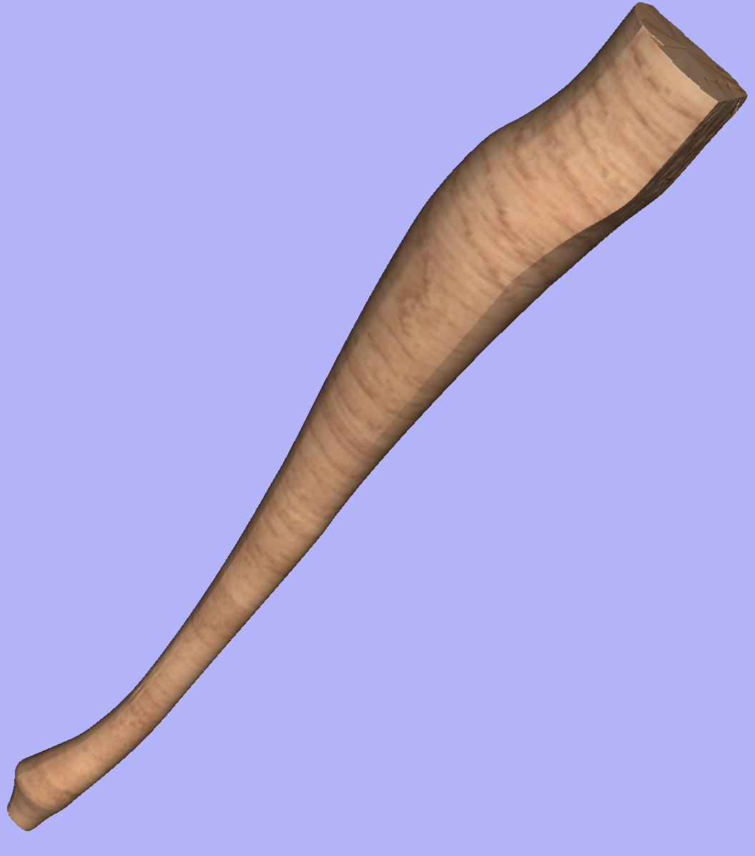
This section will present the process of importing the Full-3D STL model into rotary project, using a table leg as an example.
Overview
There are two basic use cases when importing an external model into the rotary job. The first case involves bringing a model designed for this particular job in another software. Thus the dimensions of the imported piece may already be correct and it can be desired to use them for the size of project. The second use case is when importing a stock model that would have to be scaled to fit on particular machine.
Aspire uses following workflow that covers both of those cases:
- Setting-up rotary project
- Choosing file for import
- Orientating the model in material block
- Scaling the model
- Finishing the import
Setting up a rotary project
Create a new job using the Job Setup form. It is important to set the job type as rotary to ensure a proper import tool is used in the next step.
If the dimensions of the project are already known, they could be specified directly.
If it is desired to fit the model to a given machine or stock available, set both the diameter and length to maximum. During import the model will be scaled to those limits.
If it is desired to use the imported model size, any size can be specified at this time. During the model import the project can be automatically resized to match the model dimensions.
In this example it was desired to fit the model into a specific stock size with a Diameter of 4 inches and a Length of 12 inches. XY origin was set to centre.
Importing the file and orientating it
To start the importing process, use Import a Component or 3D Model tool from the Modelling tab
Make sure that the Imported model type is set to Full 3D model .
The first step is to position the imported model within the material. This step is necessary as this information is not present in the imported file. When the model was opened, the import tool chose the initial orientation, as can be seen below.
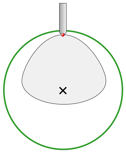
To help with orientating the model, the software displays a blue bounding cylinder. This cylinder has the rotation axis aligned with that defined for the material block and thus can be used as a reference. Its size is just big enough to contain the imported model at the current orientation. When the model orientation is changed, this blue cylinder will shrink or grow so it always contains the model. At this stage its exact dimensions are not important, as we are only interested in positioning the model correctly.
The software also highlights the rotation axis in red. This is particularly important when importing bended models. It is currently not possible to represent areas of model that are entirely below or above the rotation axis. This is the case in the example shown here. If the model was imported as is, the distortion would be created as can be seen below. Therefore it is important to position the model in a way such that the rotation axis is contained within the model.
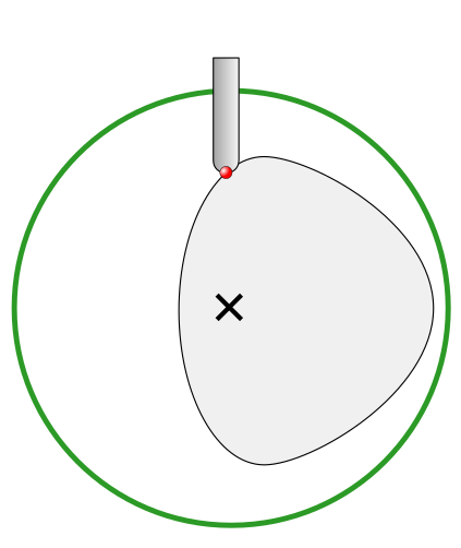
The last guiding element displayed by the software is the red half arrow on the side of the cylinder. This arrow is indicating the position that corresponds to the center of the wrapped dimension in the 2D view. In this example the model is orientated in such a way, that front of the leg would be placed on side of the 2D view, rather than centre. Thus it is better to rotate model so this arrow points to the front of the imported model.
The import tool provides a few ways of adjusting the model orientation. The most basic one is the Initial Orientation. This can be used to roughly align the model with the rotation axis. This can also be combined with the Rotation about Z Axis.In this example the tool chose Left with no rotation. In order to align the front of the leg with the red arrow, one could use the Front and -90 as the Rotation about Z Axis.
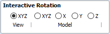
Once the initial orientation is decided, further adjustments can be made using the Interactive Rotation. The default option - XYZ View - disables the interactive rotation. That means that the 3D view can be twiddled with a mouse. Selecting other options enables the rotation around the specified axis.
In this example, instead of changing the initial orientation to align the front of the leg with the red arrow, one could select X Model option and rotate the piece manually. When selecting single axis rotation, the 3D view will be adjusted to show that axis pointing towards the screen. If any mistake is made, it is possible to undo rotation using Ctrl+ Z
Notice that whenever the part is rotated, it is always centered in the cylinder. In this example it is not desired, since we need the rotation axis to be contained within the model. In order to move the model in relation to the rotation axis, one can use the Rotation Axis Movement
Similarly to the previously described tool, when Rotation Axis Movement is set to Off, the 3D view can be panned
Correctly positioning the model for importing may require a combination of the Rotation Axis Movement and the Interactive Rotation to achieve desired results with models that bend. It is important to make sure that rotation axis is hidden in order to avoid distortion. However it is also desirable to have the rotation axis being in the center of each segment of the piece to ensure tool has angle close to the optimal during machining. Usually it is also useful to rotate the model in view around the axis after the adjustment, as this allows us to inspect the model from each side without the need to disable the Interactive Rotation before changing the viewing angle.
It is important to understand that Aspire does not support 4-axis machining. That means that while the machined piece can be rotated and tool moves along the rotation axis and in the Z direction, it is not possible to move the tool in the wrapped dimension and thus the tool is always above the rotation axis and cannot be moved to the side.
This limitation is shown below. The first picture presents correct machining of the point. If the tool moves to another location though, the angle will be incorrect and even worse, the tool side will be touching the stock.
Scaling imported model
Once model has been positioned as desired, its size can be taken into account.
By default the tool will assume that imported model is using the same units as the project. If that is not the case, model units can be switched. In this example project was set-up in inches, while imported model was designed in mm. After switching model becomes considerably smaller and a red cylinder, representing current material block is shown, as can be seen below.
At this point it is possible to specify the model size, in terms of diameter and length. This can be done manually by typing desired dimensions, or by fitting to material. If Lock ratio option is selected, the ratio between diameter and length is kept. One can also tick Resize material block option. If it is selected, the material block will be scaled to match current size of the model, after OK is clicked.
If it is desired to use model size as material block size, one can just make sure units are correct, then tick Resize material block option and press OK.
If it is desired for the model to fit material, one could click Scale model to fit material and tick Resize material block.
In this example model was fitted to material. Since in this case length of the piece is limiting factor and lock ratio is maintained, this results in model having considerably smaller diameter than material block. Hence Resize material block option was ticked.
Finishing import
After pressing OK the model will be imported as a component. It is possible to modify it as any other component or add pieces of decorative clipart onto its surface if desired.
It is important to keep in mind the distortion caused by the wrapping process. That means that wrapped toolpaths will match flat toolpaths only at the surface of the blank. The closer to the rotation axis (i.e. deeper) the toolpath is, the more it will be 'compressed'. This fact have a profound implication for 3D toolpaths. Consider the example shown below.
As can be seen if there is substantial difference in diameter in different parts of model, generating one 3D toolpath for whole model will result in wrapped toolpath being overly compressed. Thus it is usually better to create boundaries of regions with significantly different diameter and generate separate toolpaths using correct settings for each diameter.
Importing Flat Models
This section will present a process of importing Flat STL model into rotary project. Flat models are similar to decorative clipart pieces provided with Aspire and are supposed to be placed on the surface of modelled shape.
To start the importing process, use Import a Component or 3D Model tool from the Modelling tab
Make sure that Imported model type is set to Flat model
Again the first step is to select proper orientation of model. The tool will chose initial orientation and display model in the red material box. This box corresponds to the 'unwrapped' material block and its thickness is equal to half of the specified diameter of the blank.
If model is not oriented correctly, that is, does not lie flat on the bottom of the material box, as can be seen above, orientation have to be adjusted. To do that one can change Initial Orientation option and/or Rotation about Z Axis.
If imported model is not aligned with any of the axes, it may be necessary to use Interactive Rotation.The default option - XYZ View - disables interactive rotation. That means that 3D view can be twiddled with a mouse. Selecting other options enables rotation around specified axis.
Each rotation can be undone by pressing Ctrl+ Z.
Once model is properly orientated, units conversion can be performed. By default the tool will assume that imported model is using the same units as the project. If that is not the case, model units can be switched.
There is also model scaling option included. When Lock ratio option is selected, the ratio between X, Y and Z lengths are kept. Note that once model is imported, it will be added to project as a component. Hence correct placement, rotation and sizing can be performed later, after model is imported.
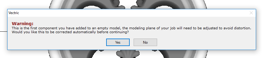
If the project does not contain any models yet, following message will be displayed:
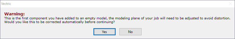
Typically you could simply click Yes.The more detailed explanation about modelling plane adjustment has been provided in Modelling 3D rotary projects
Simple Rotary Modelling using 2D Toolpaths
Creating vectors for a basic column
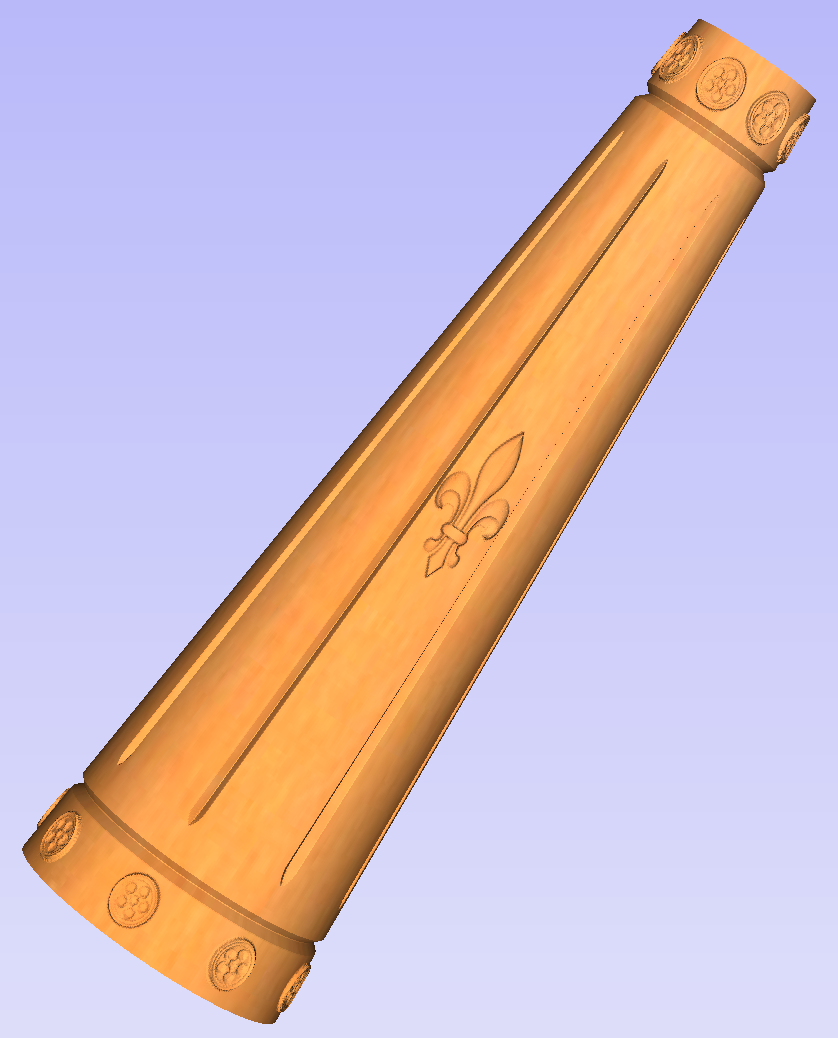
This section will show how to create a simple column, using the profile and fluting toolpaths.
Start by creating a new rotary job. Please note that settings shown here are only an example and should be adapted to match your machine setup and available material.
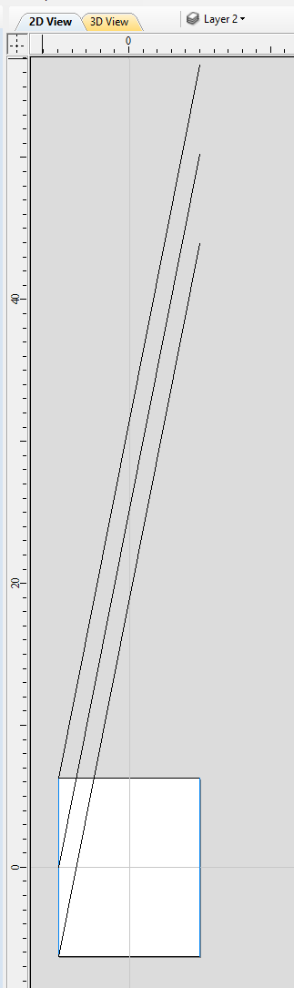
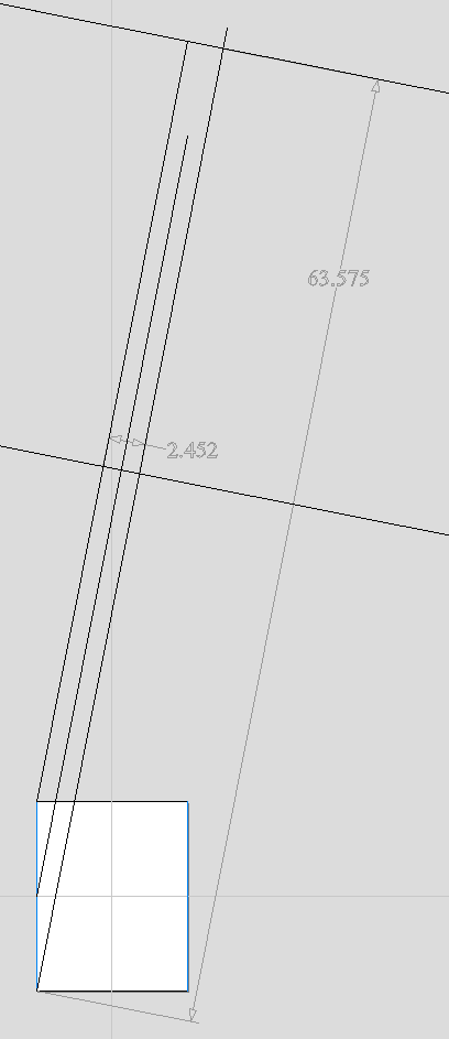
In this example the blank will rotate around X axis. We will refer to it as the rotation axis. The axis that will be wrapped is the Y axis. We will refer to it as the wrapped axis. That means that the top and bottom boundaries of the 2D workspace will actually coincide. We will refer to them as the wrapped boundaries.
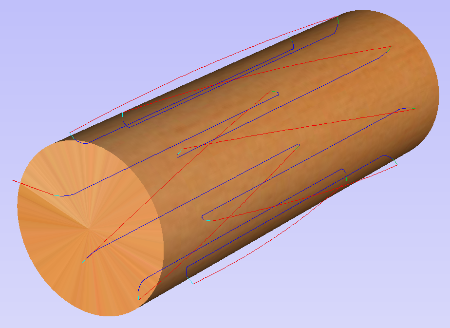
First, create the cove vectors using Draw Line/Polyline tool. Those will run along the wrapped axis at both ends of the design. Snapping may be useful to ensure that the created line starts and ends at the wrapped boundaries.
In this example the coves were placed 1 inch from the job boundaries, leaving 10 inches in the middle for the flutes. The flutes will run along rotation axis. Assuming 0.5 inch gap between the cove and the beginning of the flute, the flutes will have the length of 9 inches. This example will use 8 flutes.
To start, create a line parallel to rotation axis that is 9 inches long. Now select the created flute vector and then select one of the cove vectors while holding down Shift. Then use Copy Along Vectors tool to create 9 copies. The original flute vector may now be removed as it is no longer necessary. Note that first and last copy are both created on wrapped boundaries. That means they will coincide, so one of them can be removed. As the last step select all flute vectors and press F9 to place them in the center of design.
Creating rotary toolpaths
The process of creating 2D rotary toolpaths is very similar to creating toolpaths for Single - and Double - models. This example will use the profile toolpath on the cove vectors. To create the toolpath, select the cove vectors and click on the Profile Toolpath from
To create the toolpath for the flutes, select the flute vectors and click on the Fluting Toolpath. This Example used a 1 inch 90deg V-Bit set to Flute Depth 0.2 and using the Ramp at Start and End and Ramp Type Smooth options. Ramp length was set to 0.25 inches. Both toolpaths can be seen below.
Simulating and saving toolpaths
It is time to simulate toolpaths using Preview Toolpaths. If the option to animate the preview is selected, the simulation will be visualized in flat mode. Once the simulation is complete, the wrapped rotary view will be turned back on automatically.
Contrary to single - and double - sided simulation, rotary simulation is not 100% accurate. For example round holes will appear in rotary view as oval ones, but obviously will be round when part is actually machined.
Although the design can be considered to be finished, in practice it is useful to be able to cut-out the remaining stock. This can be realized by making the design slightly longer and adding profile cuts. In this example the blank length was extended by 2 inches using the Job Setup . Existing vectors can be recentered using F9After that the existing toolpaths have to be recalculated.
The cut-out vectors can be created in the same way as cove vectors. Two extra profiling toolpaths can be created using the suitable End Mill. In this example we used a tab with a 0.5 inch diameter. In order to achieve that, the user can type the following in the Cut Depth box: z-0.25 and then press = and the software will substitute the result of the calculation. Variable 'z' used in the formula will be substituted by the radius of the blank automatically by software. It is also important to specify Machine Vectors Outside/Right or Machine Vectors Inside/Left as appropriate. The cut-out toolpaths and the resulting simulation can been shown below.
The final step is to save the toolpaths in a format acceptable by your machine. Use the Save Toolpaths and select the wrapped post-processor matching your machine.
Note
Tools and values presented in this example are for illustrative purposes only. Size of tools, feed rate, tabs diameter etc. have to be adapted to the material and machine used to ensure safe and accurate machining.
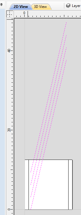
Spiral toolpaths
This section will explain how to create and simulate spiral toolpaths.
One way of thinking about spiral toolpaths is to imagine a long, narrow strip of fabric. Such a strip can be wrapped around a roll at a certain angle. In order to create a toolpath that wraps around the blank multiple times, one can create a long vector at a certain angle. Such a vector is an equivalent to the strip of fabric when it is unwrapped from the roll.
Although such a toolpath will exceed the 2D workspace of the rotary job, thanks to the wrapping process during both simulation and machining the toolpath will actually stay within material boundaries.
The most crucial part of designing spiral vectors is to determine the right angle and length of the line that would result in a given number of wraps. Suppose one would like to modify a simple column design to use spiral flutes, rather than parallel to rotation axis. The following example will use flutes wrapping 3 times each, but the method can be adapted to any other number.
All but one of the existing flute vectors can be removed. Select the Draw Line/Polyline and start a new line by clicking at one end of the existing flute. This line needs to be made along the wrapped axis with the length being 3 times the circumference of the job. In this example that means typing 90 into the Angle box and typing y * 3 into the Length box and pressing =. If the wrapped axis is not the Y axis, but rather the X axis, then the above formula should be x * 3.
Now one can simply draw a line connecting to the other end of the original flute vector and the newly created one. Using Copy Along Vectors tool this single flute may be copied in the way described earlier. In this example 4 spiral flutes were created, as can be seen below.
Once the flute vectors are ready, the toolpath can be created again using the Fluting Toolpath. An important thing to note, is the difference between the appearance of spiral toolpaths in the wrapped and flat view. By clicking on Auto Wrapping one can switch from wrapped rotary view to flat view and back again.
As can be seen above, in the flat view the toolpaths will follow the vectors and extend beyond the job boundaries. On the other hand the wrapped view, presented below, will display the toolpaths spiralling around the blank.
This was just a brief overview of general 2D workflow for rotary machining. Remember to also take a look at video tutorials dedicated to rotary machining, which are accessible from the Tutorial Video Browser link when the application first starts.
Modelling 3D Rotary Projects
Elaborating 2D designs with 3D clipart pieces
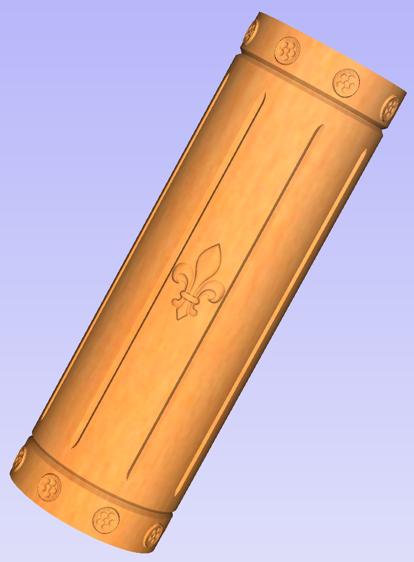
This section will present how to add 3D clipart to basic fluted column presented in Simple rotary modelling using 2D toolpaths.
A simple way to start with 3D rotary models is to use add pieces of decorative clipart that is provided with Aspire. This process is very similar to adding clipart to single - or double - sided project, however there are some additional considerations that are specific to wrapped rotary machining.
To start, switch to the Clipart tab. Then choose a piece of clipart and drag and drop it into the workspace. Aspirewill show following message:
To understand this message, we need to consider the flat view of our model, after importing the clipart. Flat view can be accessed by clicking Auto Wrapping button.
As can be seen, the model contains only the selected decorative piece on the flat plane. Although the column is obviously a cylindrical solid, so far we only used 2D toolpaths to carve details on the surface of cylinder. So the fact that machined piece is a cylindrical solid, derives only from fact that the blank is a cylindrical solid itself. Aspireallows the 3D model to also describe a solid body.
In this example the intent is to only place a decorative piece on the surface, rather than define body of the column. Aspirecan see that we did not model a body and we are placing a piece of clipart, that is likely to be placed at the surface. By responding 'Yes' to the message we can confirm that it is our intent to use the component to decorate a surface.
Note
The above message is only displayed when the 3D model is empty. Regardless of user choice, this message will not be displayed again for this project.
More clipart can be placed as desired. Then the 3D view can be inspected. Once design is finished it is time to create toolpaths. In order to create 3D roughing toolpath, use the 3D Roughing Toolpath. Then create 3D finishing toolpath, using 3D Finish Toolpath. Select settings that are most appropriate for given application, while remembering which axis is rotating. The choice of axis may be particularly important if rotation axis speed is slower than linear axis.
In this example the decorative clipart that was added was not recessed. That means that after 3D machining the flat areas around clipart will be recessed due to clipart 'standing out' of the flat surface. Therefore existing 2D toolpaths needs to be projected. This can be accomplished by selecting Project toolpath onto 3D model option and recalculating the toolpaths.
Making a tapered column
This section will explain how to make a tapered column by modifying the basic design from previous section.
So far only the surface details were modelled. In order to make a tapered shape, we need to model 'body' of the shape in addition to surface details. For that purpose, zero plane component can be used. It is added automatically for rotary jobs.
Double-click the zero plane component to open Component Properties. Enter 0.8 in the Base Height box. Select Tilt option. Click Set button in Tilt section, then switch to 2D view and then click in the middle left and then in the middle right. Set the angle to 3 degrees.
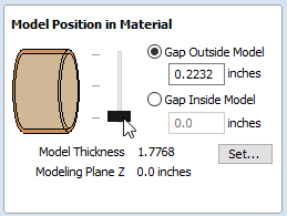
Since the modelling plane was adjusted for placing component on the surface, it needs to be adjusted again, so the component body is not 'inflated'. To do that open the Material Setup form. Adjust modelling plane by moving the slider down, until the Gap Inside Model is 0.
After modelling a tapered shape, the 3D model of column will have a desired shape. However clipart pieces in the narrower parts have been distorted, as can be seen below. To fix that, one needs to stretch the components in the wrapped dimension, to compensate for distortion.
The distortion that has been demonstrated above, applies also to toolpaths. That means that wrapped toolpaths will match flat toolpaths only at the surface of the blank. The closer to the rotation axis (i.e. deeper) the toolpath is, the more it will be 'compressed'. This fact have a profound implication for 3D toolpaths. Consider the example shown below.
As can be seen if there is substantial difference in diameter in different parts of model, generating one 3D toolpath for whole model will result in wrapped toolpath being overly compressed. Thus it is usually better to create boundaries of regions with significantly different diameter and generate separate toolpaths using correct settings for each diameter.
Modelling turned shapes
This section will present a basic technique for creating turned shapes.
Modelling turned shapes is quite easy. It requires a vector representing a profile of the desired shape and a Two Rail Sweep tool.
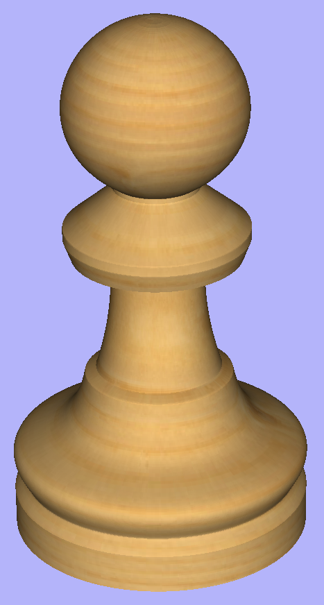
To start, create a new rotary job. Then either draw a profile using available drawing tools or import profile vector. This example used a chess pawn profile, as can be seen below.
Open the Two Rail Sweep tool. When the rotary job is created, the software inserts a special layer called '2Rail Sweep Rails'. It contains two blue lines on the sides of the job, that are perpendicular to the rotation axis.
Select both of those rails and click the Use Selection button. The rails will then be highlighted. Then select the profile vector and click apply. Inspect the 3D view to verify the results.
Modelling cross section
This section will explain how to model desired shape using Vector Unwrapper.
The Vector Unwrapper is useful when rather than modelling a profile along the rotation axis, it is more intuitive to specify a desired cross section. The tool transforms a vector, representing a cross section, into a profile vector that can be subsequently used with Two Rail Sweep tool.
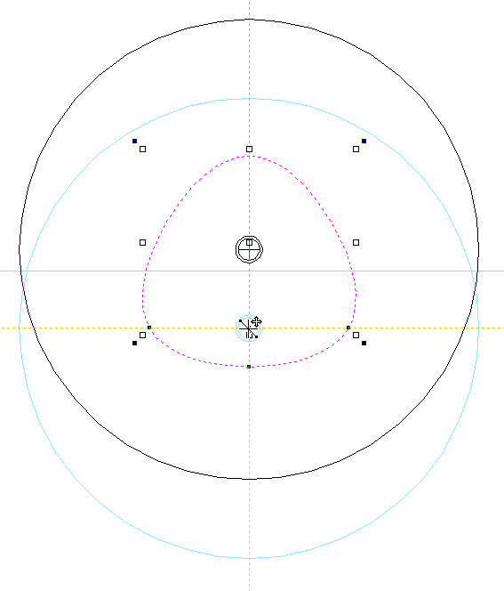
Suppose we would like to create a hexagonal-shaped column. Let's start by creating a new rotary job. In this example job has a diameter of 6 inches and is 20 inches long. X axis is the rotation axis and Z origin has been placed on the cylinder axis.
We need to create a hexagon using Draw Polygon tool. This vector will serve as a cross section and can be placed anywhere in the 2D view. In this example the material block diameter is 6 inches, so the radius of the shape cannot exceed 3 inches.
When the shape is created, select it and open Vector Unwrapper. The tool will display a crosshair in place where the rotation axis is crossing the profile and a circle with the diameter of the material block. This will help you determine whether the shape with such cross profile will fit in current material block.
In this example, the Use Center of contour option was used. That means that rotation axis will be placed in the centre of vector's bounding box. One can also tick Simplify unwrapped vectors option to fit bezier curves, instead of using series of very short line segments. After apply is pressed, the unwrapped version of the selected cross section will be created, as have been shown below.
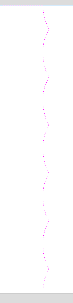
This example shows the unwrapped vector for a cylinder rotating around the X axis. If your rotary axis is aligned along Y the unwrapped vector will be horizontal. It is worth noting that unwrapped profile have 'legs' on each end. Those are needed to ensure that correct height will be used in the next step.
The tool automatically creates layer called 'Unwrapped Vectors Drive Rails' on which it places two blue line vectors on job sides, parallel to the rotation axis. In order to extrude the profile, open the Two Rail Sweep tool. Then select top and then bottom rail (left and right when Y axis is rotation axis) and confirm selection by clicking Use Selection button. The rails will now be highlighted. Now click on unwrapped vector and press apply. The 3D view will show a hexagonal column, that can be seen at the beginning of this section.
Modeling Plane
The desired cross-section will only be achieved if modelling plane is positioned in cylinder centre. That means that Gap Inside Model is reported as 0 in Material Setup form. Otherwise the resulting model will have incorrect diameter and the cross section will become rounded.
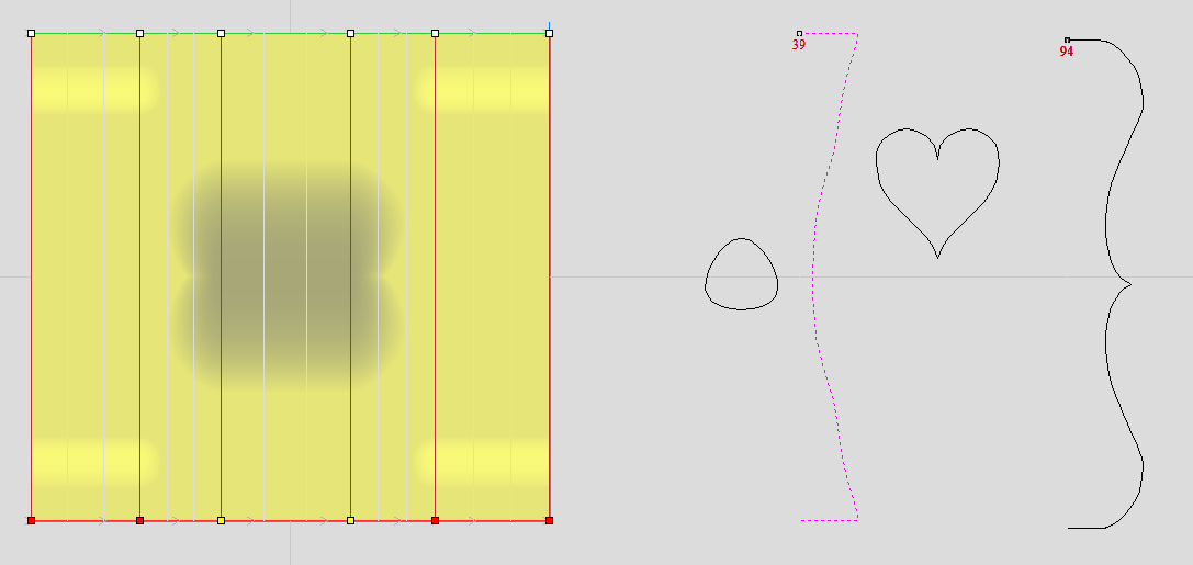
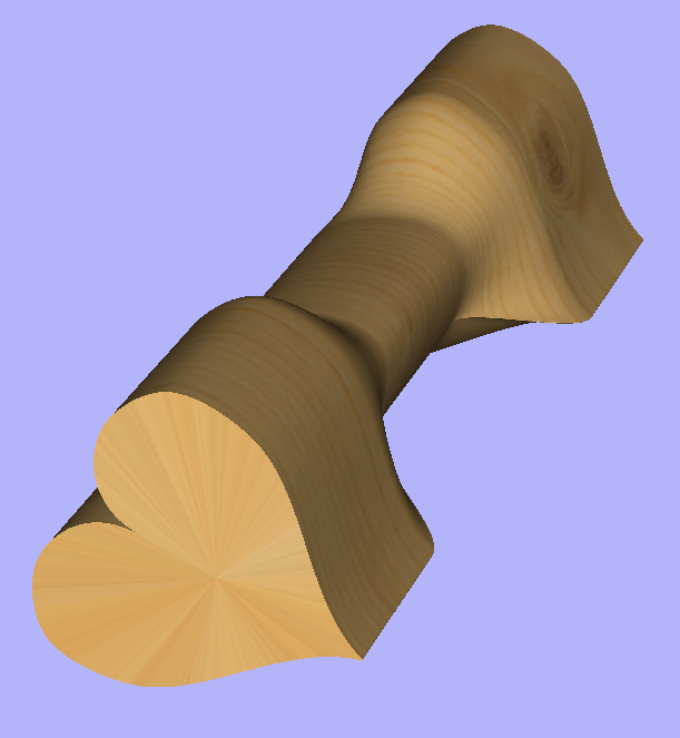
The Vector unwrapper is not restricted to simple shapes. In principle it is always possible to use convex shapes and certain concave shapes. The example below shows a heart profile unwrapped.
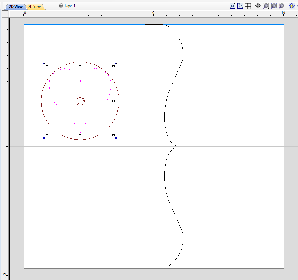
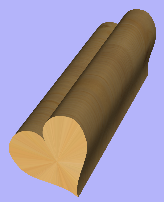
If cross section in question is concave, one could imagine straight line starting in the center of the shape and touching a point on the boundary. If the second points keeps travelling along the boundary and each line is not crossing another point on the boundary, then it is possible to use this cross section. If the line does cross more than one point on the boundary, this part of the cross section will not be represented correctly.
All the examples so far used a single cross section. However it is also possible to use multiple cross sections.
Let's take another cross section and open Vector Unwrapper. Then drag the rotation axis handle a bit down from the center. If snapping is enabled, it can be used to help position the rotation center, as can be seen below.
Once we have another unwrapped cross section, it is possible to use both during Two Rail Sweep. For example unwrapped heart profile can be placed twice on the left and twice on the right. The second unwrapped profile can be placed twice in the middle. Such arrangement may result in shape morphing, as can be seen below.
Advanced Modelling of 3D Rotary Projects
Modelling 3D spiral features
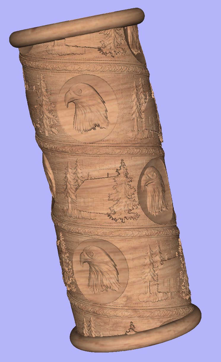
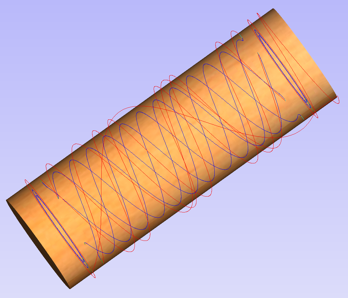
In this section we will show how to use level-wrapping feature to wrap a design in spiral manner around a column.
The workflow for creating spiral toolpaths has been presented in the Simple rotary modelling using 2D toolpaths chapter. The basic idea involved creating a line at a proper angle to the rotation axis, that exceeded the 2D boundaries. When 2D toolpath is created based on such a line, it will be wrapped around material cylinder, creating a spiral.
This guide will build on that basic idea. The task is to create a horizontal strip with desired pattern and then wrap it like a ribbon around the cylinder.
To help with that task, it is important to create some helpful vectors first. We need to create lines, that will become boundaries of our strip. In this example the strip was being wrapped four times around full length of material. This example assumes that rotation axis is parallel to X axis.
To start, select Draw Line/Polyline tool and draw a horizontal line at the bottom of the job from left to right. If it is desired for the spiral pattern to only fill part of the cylinder length, this horizontal line should be drawn only in th desired location. While the drawing tool is still active, type 90 into Angle box and type y * 4 into Length box and pressing =. We used y * 4 formula so the strip will wrap 4 times. Then press Add button to add a vertical segment.
Now, start a new line that connects the horizontal and vertical lines, forming a triangle. Once this line is created, horizontal and vertical lines can be removed.
The line that we just created will form a bottom of the strip. Now copy this line and place line so its bottom left end coincides with top left corner of the 2D job. This line will form a top of the strip. Then make another copy and place it in the middle. This middle line will be used later to position our design within strip. All three lines have been shown below.
Next step is to find out the required length and width of the strip. We will need a few extra vectors to accomplish that.
Let's copy one of the created three lines and rotate by 90 degrees, to get a line that is perpendicular to the strip. Then place it in such way so it crosses the strip. This will help us measure the width.
Then copy the perpendicular line and place it so it touches the top line. Then extend the bottom line, until it crosses the perpendicular line we just added. This will help us measure the length of the strip.
The easiest way to achieve that, is to create a textured component. To do that, select the design in the component tree and activate the Create Texture Area tool. This example used the default settings of the tool. The tool will create a new component that will fill the whole 2D job boundaries. The component itself will be filled with the design in tiled manner. Now use the Set Size tool to resize textured component to match the strip size.
Now the component have to be rotated and moved to fit between the lines you have drawn at the beginning. This process can be made easier by utilizing Copy Along Vectors tool. To proceed, activate the tool and select the textured component first, then select the middle line in the strip while holding Shift. Make sure that Align objects to curve option is selected and use Number of copies option. Since our strip has already have a correct size, we only need one copy. However the tool would place the middle of our component at the beginning of the line only. If you enter 3 as the number of copies, then the tool will place two copies of component at each end and in the middle. Afterwards the copies at the ends can be simply deleted. The picture below shows the strip in the 3D view after being correctly positioned.
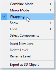
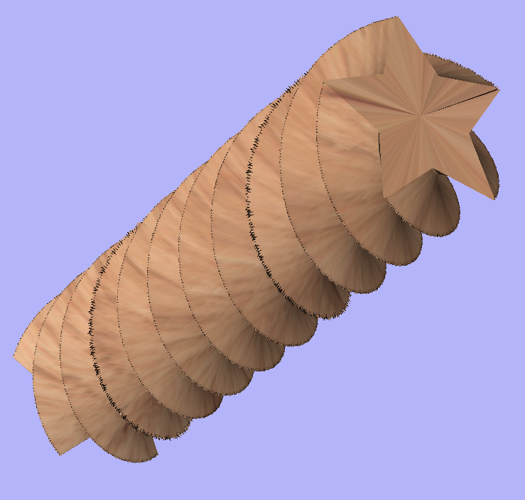
As can be seen, the strip disappears as soon as it leaves the material boundaries. In order to make it wrap around, we need to create a new level in the component tree and move the texture component into it. Then right click on the newly created level and right click. From the pop-up menu select wrapping. After that wrapping will occur.
Note:
Wrapping can be enabled on any level in component tree and combined with mirror mode. If the level wraps on itself, then intersecting areas will be merged regardless of level's combine mode. If it is desired to create e.g. a woven pattern, then place left-hand spiralled component and right-hand spiralled components in different separate levels, both with wrapping enabled.
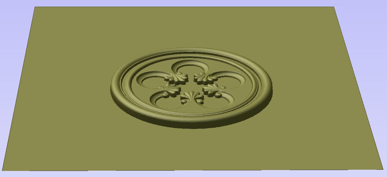
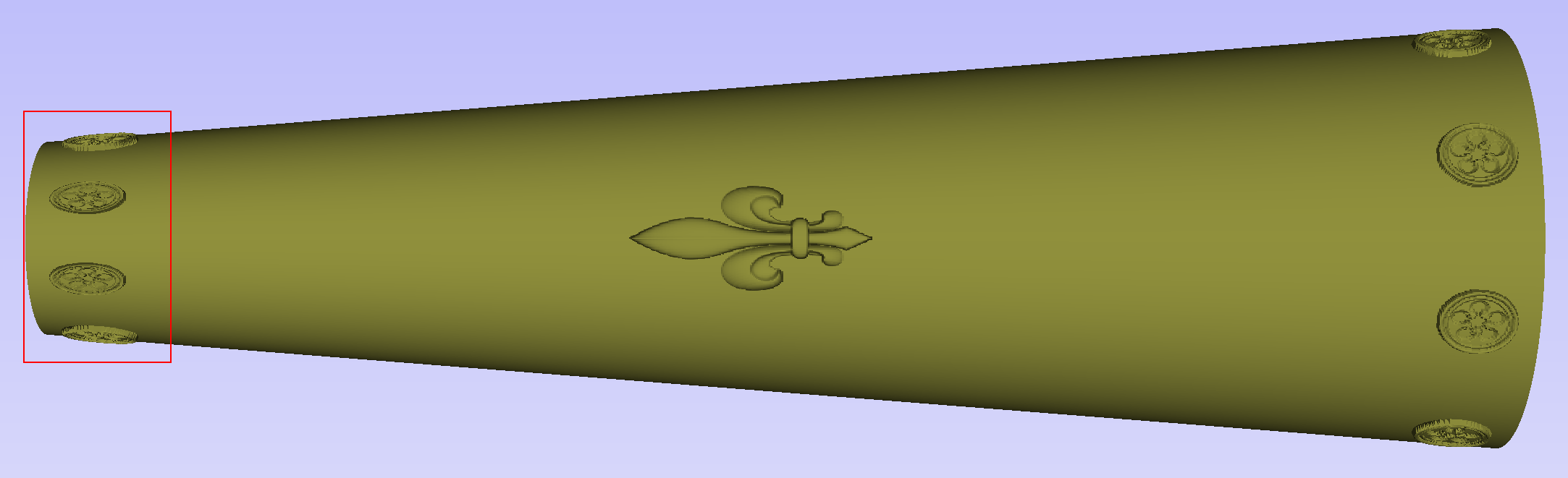
The last step is to make column endings. For that purpose the third level was created, with Combine Mode set to Merge. This way the spiral pattern will be 'hidden' at the ends. A circular 3D tab clipart was placed at each end, and stretch vertically to match the job boundaries.
Modelling twisted shapes
This section will show how to create twisted shapes, using a combination of level-wrapping and Vector Unwrapper tool.
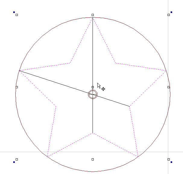
In this example a new rotary job was created, with a diameter of 6 inches and length of 20 inches, rotating around X axis. To start, we need a cross-section vector. In this example a 5-armed star was used. To create a star, we can use Draw Star tool. This example used Outer Radius of 3 inches, to match the radius of the material.
The next step is to unwrap the cross section. In the case of the star however, the center is not the same as center of star's bounding box. To find the real center, one can draw a line from two of the star corners. Then open Vector Unwrapper and select the star. Then drag rotation center and snap it to the intersection of the lines, as can be seen below.
Once the star is unwrapped, we need to create rails, that will make spiral when wrapped. To do that, select Draw Line/Polyline tool and draw a horizontal line at the bottom of the job from left to right. While the drawing tool is still active, type 90 into Angle box and type y * 2 into Length box and pressing =. We used y * 2 formula so the star will make 2 revolutions Then press button to add a vertical segment. Finally, start a new line that connects the horizontal and vertical lines, forming a triangle. Once this line is created, our horizontal and vertical lines can be removed.
Next step is to copy the line and place it so its bottom left end coincides with top left corner of 2D job.
Once the the rails are ready, one could use a Two Rails Sweep tool. However, since rails exceeds the 2D job boundaries, the created sweep will be cropped as soon as those boundaries are exceeded.
To overcome that, select both rails, open Draw Rectangle tool and press . This will create a bounding box containing the rails. Now, write done the size of the box and save current project. Then create a new single-sided project with the slightly bigger than the bounding box. Use the Import Vectors option from the main menu and select the previously saved file. Now select the rails and press F9 to center them.
Now use Two Rail Sweep tool. When component is ready, save the file.
Now re-open the original rotary project. Use Import Component and select the single-sided project created in the step above. Move the component to the desired location. Then, create a new level, move the component there and enable wrapping.
Using single-sided modelling tools
This section will present how to use single-sided modelling techniques in rotary projects.
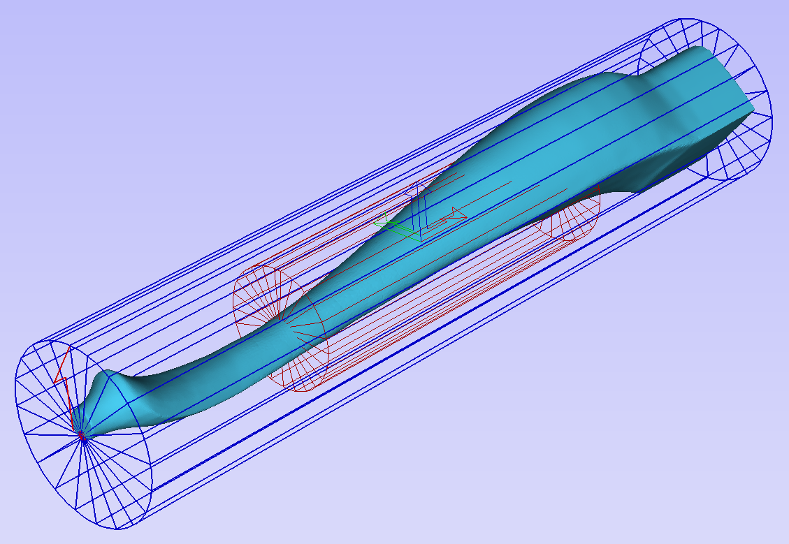
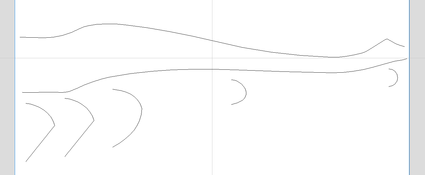
Users familiar with modelling techniques used in single-sided projects may find them more convenient for modelling certain shapes. This example uses two vectors, representing side cross section of the table leg and a few of half cross sections for different parts of the table leg. Those vectors are presented below.
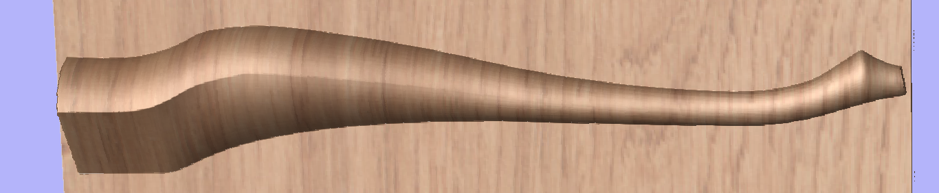
One can simply treat the side cross section as rails and use the Two Rail Sweep tool, placing the half cross sections at appropriate locations. This way half of the leg can be modelled very quickly, with the result that can be seen below (using flat 3D view).
In order to use the created model in a rotary project, we need to export and then import it back. Although it is possible to do this with two sessions of Aspire, it can also be done within a single session with rotary project. To export the leg model, make sure no other components are visible (including the automatically added zero plane) and open the Export Model tool while holding down Shift. Pressing Shift allows to open the export tool in single-sided, rather than rotary mode.
Since half of the leg was modelled, Close with inverted front option can be used. The resulting STL mesh can be seen below.
Once component is exported, it can be re-imported as Full 3D model. The model will have a seam, in the place were two halfs were merged. This can be removed using smoothing function of the Sculpting tool.
Postprozessor-Bearbeitung
Was macht ein Postprozessor?
Der Postprozessor ist der Abschnitt eines Programms, der die XYZ-Koordinaten für die Werkzeugbewegungen in ein Format umwandelt, das für einen bestimmten Router oder Fräswerkzeug geeignet ist. Dieses Dokument beschreibt im Detail, wie Sie die Konfigurationsdateien erstellen und bearbeiten, die die Ausgabe des Programms auf eine bestimmte Maschinensteuerung anpassen.
Im Folgenden finden Sie Abschnitte eines typischen Programms, das sowohl in G-Code als auch in HPGL verarbeitet wurde.
Ausgabe in G-Code
T1 M6
G17
G0 Z4.5000
G0 X0.0000 Y0.0000 S12000 M3
G0 X2.4567 Y7.8342 Z0.2500
G1 Z-0.0500 F5.0
G3 X3.3784 Y8.7559 I0.0000 J0.9218 F66.0
G3 X2.4567 Y9.6777 I-0.9218 J0.0000
G3 X1.5349 Y8.7559 I0.0000 J-0.9218
Ausgabe in HPGL
IN;PA;
PU2496,7960;
PD2496,7960;
AA2496,8896,90.000
AA2496,8896,90.000
AA2496,8896,90.000
AA2496,8896,90.000
PU2496,7960;
PU2496,6096;
Hersteller von Maschinensteuerungen passen das für bestimmte Maschinen erforderliche Dateiformat oft an, um die Steuerung auf die individuellen Eigenschaften der jeweiligen Maschine zu optimieren.
Der Vectric-Postprozessor verwendet einfache textbasierte Konfigurationsdateien, mit denen die Benutzer eine Konfigurationsdatei genau zuschneiden können, sollten sie dies wünschen.
Postprozessor-Abschnitte
Die Vectric-Postprozessoren sind für größere Klarheit in Abschnitte untergliedert. Schreiben Sie Ihre Postprozessoren auf eine ähnliche Weise, um Debugging zu vermeiden.
Dateikommentare
Ein Abschnitt, in dem Sie den Postprozessor beschreiben und Änderungen am Postprozessor dokumentieren können. Jede Zeile ist ein Kommentar und beginnt mit den Zeichen „+“ oder „|“.
+ Verlauf
+ Wer Wann Was
+ ======== ========== ===========================
+ Tony 14.07.2006 Geschrieben
+ Mark 26.08.2008 ATC-Befehle zusammengefasst, Spindelstopp bei TC
+================================================
Globale Dateianweisungen
Anweisungen sind Einheiten, die entweder nur einmalig verwendet werden oder in der gesamten Datei statische Werte haben. Schreiben Sie die Namen der Anweisungen zur Verdeutlichung in Großbuchstaben.
Anweisung | Ergebnis |
|---|---|
| Der Name, der in der Liste der Postprozessoren angezeigt wird |
| Die Erweiterung für diese Datei |
| Die Einheiten, die diese Datei ausgibt (INCHES oder MM) |
| Der Hersteller des Fräswerkzeugs hat einen Treiber bereitgestellt (im Normalfall einen Druckertreiber), der die NC-Dateiausgabe direkt akzeptieren kann (Ein Beispiel finden Sie unter Generic HPCL_Arcs.pp) |
| Gibt an, dass Eintauchbewegungen auf die Eintauchhöhe (Z2) (im Formular Materialeinrichtung festgelegt) schnelle Bewegungen sind |
| Die Steuersoftware verwendet eine Dokumentschnittstelle, die NC-Dateiausgaben direkt akzeptieren kann. |
| Die Bewegungen auf der Y-Achse werden um einen Zylinder mit dem angegebenen Durchmesser gewickelt. Die "Y"-Werte werden als "A" ausgegeben. |
| Die Bewegungen auf der X-Achse werden um einen Zylinder mit dem angegebenen Durchmesser gewickelt. Die "X"-Werte werden als "B" ausgegeben. |
| Die Spindeldrehzahl für diese Maschine wird als Bereich von Ganzzahlen zwischen 1 und 15 ausgegeben, welche für die tatsächliche Spindeldrehzahl in U/min steht (im genannten Beispiel zwischen 4500 und 15.000 U/min). Ein Beispiel finden Sie unter: Roland_MDX-40_mm.pp |
| Über diesen Befehl können Sie eine Zeichenausgabe innerhalb der Variable (zum Beispiel Diese Zeichen können paarweise eingegeben werden, Original - Ersetzt. Die Steuersoftware MACH 3 verwendet zum Beispiel Klammern als Kommentartrennzeichen und erlaubt keine verschachtelten Kommentare. Die meisten Werkzeuge in der Vectric-Werkzeugdatenbank verwenden im Bereich "Name" Klammern; wenn diese Namen ausgegeben werden, würde dies in Mach3 einen Fehler verursachen. Mit dem Befehl |
| Drehen: Aktiviert / Deaktiviert die Ausgabe der Vorschubgeschwindigkeit F im Vorschubmodus mit inverser Verzögerung. In diesem Modus sollen wir die Bewegungen nacheinander ausführen, getrennt durch die Anzahl F in Minuten. In GCode wäre dies ursprünglich G93, um in den inversen Verzögerungsmodus zu wechseln, oder G94, um den Modus "Einheiten pro Minute" einzustellen. |
| Gibt an, dass dieser Postprozessor Laser-Werkzeugpfade unterstützt (bei installiertem Lasermodul). |
| Optionaler minimaler Bogenradius. Bögen, deren Radien diesen Wert unterschreiten, werden durch eine einzelne gerade Bewegung ersetzt. |
| Optionaler maximaler Bogenradius. Bögen, deren Radien diesen Wert überschreiten, werden durch Polygone ersetzt. |
POST_BASE | Eine nicht mehr unterstützte Weise, den Inhalt eines anderen Postprozessors zu erben. Weitere Informationen finden Sie auf der Seite POST_BASE Migration. |
Bandtrennungs-Support
In diesem Abschnitt wird beschrieben, auf welche Weise eine lange Werkzeugpfad-Ausgabe getrennt wird:
TAPE_SPLITTING=MAX_NUM_LINES LINE_TOL "FILENAME_FORMAT" START_INDEX INDEX_ON_FIRST_FILE
Beispielsweise würde ein Befehl:
TAPLE_SPLITTING=1000 100 "%s_%s.tap" 1 "YES"
dazu führen, dass ...
Die Ausgabe in mehrere Dateien mit maximal 1000 Zeilen (+ die erforderliche Anzahl Zeilen in der Fußzeile des Postprozessors) aufgeteilt wird. Wenn nach Zeile 900 (1000-100) eine Abhebebewegung vorgesehen ist, wird die Datei bei dieser Bewegung geteilt. Wenn die Datei mit „toolpath“ benannt ist, werden die aufgeteilten Dateien toolpath_1.tap, toolpath_2.tap usw. benannt. Die erste Werkzeugpfad-Ausgabe lautet „toolpath_1.tap“. Keine Datei wird mit „toolpath“ ohne Index benannt (durch INDEX_ON_FIRST_FILE= YES), wenn die Datei nicht kürzer als 1000 Zeilen war. In diesem Fall wird die Datei nicht aufgeteilt.
Hinweis
Bei einigen Steuerungen, für die NC-Dateien aufgeteilt werden müssen, ist auch die Zeichenanzahl für den Dateinamen begrenzt. Für sie muss die Datei beispielsweise gemäß dem MSDOS-Format 8.3 benannt werden. Dies sollte bei der Benennung der Ausgabedatei beachtet werden.
Zeilentrenner
LINE_ENDING="[13][12]"
Dezimalwerte der Zeichen, die den einzelnen Zeilen der Postprozessor-Datei angehängt werden. Üblicherweise werden für alle Steuerungen, die Textdateien im Windows- oder MSDOS-Format lesen können, [13][10] (Zeilenumbruch, Zeilenvorschub) verwendet.
Blocknummerierung
Wenn Sie der Ausgabedatei Zeilennummern hinzufügen möchten, wird die aktuelle Zeilennummer mit der Variable [N] hinzugefügt. Das Verhalten dieser Zeilennummer-Variablen wird durch die folgenden Variablen gesteuert:
Anweisung | Ergebnis |
|---|---|
| Startwert der Zeilennummerierung |
| Inkrementwert zwischen den Zeilennummern |
| Die größte ausgegebene Zeilennummer, bevor die Zählung mit dem Wert Wichtig - Bei einigen Steuerungen ist die darstellbare Zeilenanzahl begrenzt. |
Variablen
Name der Variablen | Ausgabe verwendet | Wert | Beispieldatei |
|---|---|---|---|
|
| Aktuelle Vorschubgeschwindigkeit. | Mach2_3_ATC_Arcs_inch.pp |
|
| Aktuelle Schnitt-Vorschubgeschwindigkeit. | CNCShark-USB_Arcs_inch.pp |
|
| Aktuelle Eintauchgeschwindigkeit. | CNCShark-USB_Arcs_inch.pp |
|
| Aktuelle Spindeldrehzahl in U/min. | GCode_arc_inch.pp |
|
| Aktuelle Leistungseinstellung für Strahlwerkzeuge (z. B. Laser) | grbl_mm.pp |
|
| Aktuelle Werkzeugnummer. | Mach2_3_ATC_Arcs_inch.pp |
|
| Vorherige Werkzeugnummer. | NC-Easy.pp |
|
| Zeilennummer. | Mach2_3_ATC_Arcs_inch.pp |
|
| Name des aktuellen Werkzeugs. | MaxNC_inch.pp |
|
| Text aus dem Notizfeld in ToolDB für das aktuelle Werkzeug | Busellato_Jet3006_arc_inch.pp |
|
| Name des aktuellen Werkzeugpfads. | Viccam_ATC_Arcs_inch.pp |
|
| Dateiname (durch "Werkzeugpfad(e) speichern ..." erstellt) | ez-Router_inch.pp |
|
| Ordner, in dem die Werkzeugpfaddatei gespeichert wurde. | Woodp_arc_mm.pp |
|
| Werkzeugpfad-Erweiterung. | TekcelE_Arc_ATC_3D.pp |
|
| Pfadname des Werkzeugpfadordners. | WinPC-NC_ATC_Arcs_mm.pp |
|
| Aktuelle Koordinate der Werkzeugposition auf der X-Achse. | GCode_arc_inch.pp |
|
| Aktuelle Koordinate der Werkzeugposition auf der Y-Achse. | GCode_arc_inch.pp |
|
| Aktuelle Koordinate der Werkzeugposition auf der Z-Achse. | GCode_arc_inch.pp |
|
| Aktuelle Koordinate der Werkzeugposition auf der A-Achse. | |
|
| Bogenmittelpunkt auf der X-Achse (im Verhältnis zu letzten X/Y-Position). | Mach2_3_ATC_Arcs_inch.pp |
|
| Bogenmittelpunkt auf der Y-Achse (im Verhältnis zu letzten X/Y-Position). | Mach2_3_ATC_Arcs_inch.pp |
|
| Bogenmittelpunkt auf der X-Achse (absolute Koordinaten). | Isel_arc_mm.pp |
|
| Bogenmittelpunkt auf der Y-Achse (absolute Koordinaten). | Isel_arc_mm.pp |
|
| Startposition eines Bogens auf der X-Achse. | TextOutput_Arcs_mm.pp |
|
| Startposition eines Bogens auf der Y-Achse. | TextOutput_Arcs_mm.pp |
|
| Scheitelpunkt eines Bogens auf der X-Achse (absolute Koordinaten). | TextOutput_Arcs_mm.pp |
|
| Scheitelpunkt eines Bogens auf der Y-Achse (absolute Koordinaten). | TextOutput_Arcs_mm.pp |
|
| Scheitelpunkt eines Bogens auf der X-Achse (inkrementelle Koordinaten). | TextOutput_Arcs_mm.pp |
|
| Scheitelpunkt eines Bogens auf der Y-Achse (inkrementelle Koordinaten). | TextOutput_Arcs_mm.pp |
|
| Der Radius eines Bogens. | Bosch_ATC_Arcs_mm.pp |
|
| Der Winkel eines Bogens. | Generic HPGL_Arcs.pp |
|
| Ruheposition des Werkzeugs auf der X-Achse. | CAMTech_CMC3_mm.pp |
|
| Ruheposition des Werkzeugs auf der Y-Achse. | CAMTech_CMC3_mm.pp |
|
| Ruheposition des Werkzeugs auf der Z-Achse. | CAMTech_CMC3_mm.pp |
|
| Sicherheitsabstand Z / Abstand für schnelle Bewegung. | EMC2 Arcs(inch)(*.ngc) |
|
| Durchmesser des Zylinders, um diese Achse gewickelt wird. | Mach2_3_WrapY2A_ATC_Arcs_mm.pp |
|
| Länge des Materials auf der X-Achse. | Mach2_3_ATC_Arcs_inch.pp |
|
| Länge des Materials auf der Y-Achse. | Mach2_3_ATC_Arcs_inch.pp |
|
| Länge des Materials auf der Z-Achse. | Mach2_3_ATC_Arcs_inch.pp |
|
| Mindestwert des Materials auf der X-Achse. | MaxNC_inch.pp |
|
| Mindestwert des Materials auf der Y-Achse. | MaxNC_inch.pp |
|
| Mindestwert des Materials auf der Z-Achse. | MaxNC_inch.pp |
|
| Maximalwert des Materials auf der X-Achse. | MaxNC_inch.pp |
|
| Maximalwert des Materials auf der Y-Achse. | MaxNC_inch.pp |
|
| Maximalwert des Materials auf der Z-Achse. | MaxNC_inch.pp |
|
| Ursprungsposition auf der X-Achse. | TextOutput_Arcs_mm.pp |
|
| Ursprungsposition auf der Y-Achse. | TextOutput_Arcs_mm.pp |
|
| Z-Nullpunkt, Tisch- oder Materialoberfläche. | TextOutput_Arcs_mm.pp |
|
| Ursprung auf der X- und Y-Achse. | TextOutput_Arcs_mm.pp |
|
| Liste der verwendeten Werkzeuge (in der Reihenfolge ihrer Verwendung). | Mach2_3_ATC_Arcs_inch.pp |
|
| Liste der in der Datei verwendeten Werkzeugpfade (in der Reihenfolge ihrer Verwendung). | Mach2_3_ATC_Arcs_inch.pp |
|
| Werkzeugpfad-Anmerkungen (Werkzeugpfad-Steuerungsmenü). | Mach2_3_ATC_Arcs_inch.pp |
|
| Dateianmerkungen (Bearbeiten > Anmerkungen). | Mach2_3_ATC_Arcs_inch.pp |
|
| Erstellungszeitpunkt der Datei. | Mach2_3_ATC_Arcs_inch.pp |
|
| Erstellungsdatum der Datei. | Mach2_3_ATC_Arcs_inch.pp |
|
| Haltezeit in Sekunden beim Bohren. | Mach2_3_Arcs_inch.pp |
|
| Name des Produkts für die Dateiausgabe, einschließlich Versionsnummer. | |
|
| Werkzeugdurchmesser. | |
|
| Drehen: Aktuelle inverse Verzögerungsrate. | AvidCNC_WrapX2A_G93_inch.pp |
Variablenformat
Werte für die Werkzeugposition, Vorschubgeschwindigkeit, Spindeldrehzahlen usw. werden mithilfe von Variablen in die Datei eingegeben. In der gesamten Datei werden Variablen verwendet; die Variablen werden beim Postprocessing der Datei durch den aktuellen Wert für diesen Eintrag ersetzt. Die aktuellen Werkzeugpositionen auf der X-, Y- und Z-Achse zu einem bestimmten Zeitpunkt werden beispielsweise mithilfe der Variablenausgabe [X], [Y] oder [Z] in die Datei eingesetzt.
Schreiben Sie die Namen der Variablen zur Verdeutlichung in Großbuchstaben.
Eine Variable wird folgendermaßen formatiert:
VAR VARIABLE = [VO|WO|CS|VF|MX]
Hierbei gilt:
VO= Variablenausgabe, zum Beispiel X, XF oder F.WO= Bei Ausgabe, A=Immer, C=Nur bei Änderung.CS= Zeichenstring-Ausgabe vor Wert.VF= Wertformat, legt das Format fest, in dem der Wert ausgegeben wird.MX= Multiplikatorwert.
Eine typische Variable
1 | 2 | 3 | 4 | 5 | 6 | 7 | 8 | 9 | 10 | 11 | 12 | 13 | 14 | 15 |
|---|---|---|---|---|---|---|---|---|---|---|---|---|---|---|
|
|
|
|
|
|
|
|
|
|
|
|
|
|
|
VAR- Diese Zeile ist eine Variable.- Name der Variablen.
- Gleichheitszeichen.
- Offene eckige Klammer - (Start der Variablen-Formatierungsparameter).
- Variablenkennzeichnung - also die Kennzeichnung, die mit dem Variablenwert ersetzt wird.
- Senkrechter Strich – Parametertrenner.
- A = Immer Ausgabewert, C = Ausgabewert nur bei Änderung
- Senkrechter Strich – Parametertrenner.
- Vor dem Variablenwert auszudruckender Zeichenstring.
- Senkrechter Strich – Parametertrenner.
- Optionale Formatmarkierungen – Details siehe unten.
- Wertformat – Einheiten und Anzahl der auszugebenden Dezimalstellen.
- Senkrechter Strich – Parametertrenner.
- Ausgabemultiplikator – Details siehe unten.
- Geschlossene eckige Klammer – Ende der Formatierungsparameter.
Ausgabewert formatieren
Der String für das Wertformat sollte folgendermaßen formatiert sein:
FORMAT_FLAGS FIELD_WIDTH DECIMAL_SEPARATOR DECIMAL_PLACES
Die Formatkennzeichnungen sind optional und werden nur von wenigen Steuerungen benötigt. Sie werden in Kürze beschrieben.
Feldbreite Die Feldbreite gibt die Mindestanzahl ausgegebener Zeichen an. Die Feldbreite wird normalerweise auf „1“ gesetzt. Ein größerer Wert als 1 ist normalerweise nur dann erforderlich, wenn eine Steuerung eine feste Zeichenanzahl für den Wert erwartet. In diesem Fall kann eine größere Anzahl als 1 eingegeben werden. Die eingegebene Zahl sorgt dafür, dass diese Zeichenanzahl ausgegeben wird. Die Zahl für die Feldbreite umfasst für den Ausgabewert die gesamte Fließkommazahl (einschließlich Dezimaltrennzeichen).
Dezimaltrennzeichen Das Dezimaltrennzeichen ist fast immer ein Punkt, aber manche Steuerungen erwarten an dieser Stelle ein Komma. (Ein Beispiel für einen Postprozessor, der keinen Punkt verwendet, finden Sie in der Datei: Heidenhain_inch.pp)
Dezimalstellen Die Anzahl der nach dem Dezimaltrennzeichen ausgegebenen Dezimalstellen. Die Werte werden häufig für Steuerungen im metrischen System auf 3, für Steuerungen im imperialen System auf 4 Stellen gesetzt.
Optionale Formatmarkierungen
Die Ausgabewerte können mithilfe der folgenden optionalen Formatmarkierungen weiter modifiziert werden:
Markierung | Funktion | Standard (ohne Markierung) |
|---|---|---|
| Ausgabe linksbündig ausrichten | Werte sind rechtsbündig |
| Vorzeichen "+" oder "-" für den Wert | Nur negative Werte erhalten das Vorzeichen |
| Wenn der Wert über weniger Zeichen als der gesetzte Mindestwert verfügt, erhält er vorstehende Nullen. | Dem Wert stehen Leerzeichen vor |
| Werte werden immer mit einem Trennzeichen ausgegeben (in der Praxis würde sich der Ausgabewert nur ändern, wer der Wert auf ausschließlich Ganzzahlen gesetzt wurde) | Wenn die Ausgabe auf ausschließlich Ganzzahlen gesetzt wurde, wird dem Wert kein Trennzeichen angehängt. |
Standardformatierung für Variablen
Für die meisten Werte ist ein Standardformat gesetzt (unten angegeben). Geben Sie für ein abweichendes Format die folgende Zeile in Ihren Postprozessor ein und ändern Sie die Parameter passend zu Ihrer Steuerung.
Standard | Beispiel |
|---|---|
|
Die Zeilennummer wird immer ausgegeben. Vor der Zeilennummer wird das Zeichen "N" eingefügt. Es wird als Ganzzahl ausgegeben. |
|
Die Spindeldrehzahl wird immer ausgegeben. Vor dem Wert wird das Zeichen "S" eingesetzt. Er wird als Ganzzahl ausgegeben. |
|
Die Vorschubgeschwindigkeit wird mit dem Zeichen ‚F‘ vor dem Wert ausgegeben. Der Wert wird nur bei einer Änderung ausgegeben. Der Wert wird auf eine Dezimalstelle genau ausgegeben. Hinweis In diesem Formatstring befindet sich ein optionaler zusätzlicher Parameter. Bei diesem handelt sich um einen Wertmultiplikator. |
VAR PLUNGE_RATE = [FP|A||1.0] |
Die Eintauchgeschwindigkeit wird mit dem Zeichen ‚F‘ vor dem Wert ausgegeben. Der Wert wird nur bei einer Änderung ausgegeben. Der Wert wird auf eine Dezimalstelle genau ausgegeben. Hinweis In diesem Formatstring befindet sich ein optionaler zusätzlicher Parameter. Bei diesem handelt sich um einen Wertmultiplikator. |
|
Die Schnittgeschwindigkeit wird mit dem Zeichen ‚F‘ vor dem Wert ausgegeben. Der Wert wird nur bei einer Änderung ausgegeben. Der Wert wird auf eine Dezimalstelle genau ausgegeben. Hinweis In diesem Formatstring befindet sich ein optionaler zusätzlicher Parameter. Bei diesem handelt sich um einen Wertmultiplikator. |
|
Der Positionswert wird vor dem Wert mit einem Zeichen ‚X‘ ausgegeben. Die Position wird immer ausgegeben, die Genauigkeit beträgt 3 Nachkommastellen. Dies ist üblicherweise für eine Steuerung geeignet, die eine metrische Ausgabe benötigt. Wenn Sie die Werte mit 4 Nachkommastellen ausgeben möchten, was für eine Steuerung üblich ist, die im imperialen System arbeitet, formatieren Sie die Zeile folgendermaßen.
|
|
Der Wert für die Ruheposition wird vor dem Wert mit einem Zeichen ‚X‘ ausgegeben. Die Position wird immer ausgegeben, die Genauigkeit beträgt 3 Nachkommastellen. Dies ist üblicherweise für eine Steuerung geeignet, die eine metrische Ausgabe benötigt. Wenn Sie die Werte mit 4 Nachkommastellen ausgeben möchten, was für eine Steuerung üblich ist, die im imperialen System arbeitet, formatieren Sie die Zeile folgendermaßen.
|
|
Der Wert wird vor dem Wert mit einem Zeichen ‚X‘ ausgegeben. Die Position wird immer ausgegeben, die Genauigkeit beträgt 3 Nachkommastellen. Dies ist üblicherweise für eine Steuerung geeignet, die eine metrische Ausgabe benötigt. Wenn Sie die Werte mit 4 Nachkommastellen ausgeben möchten, was für eine Steuerung üblich ist, die im imperialen System arbeitet, formatieren Sie die Zeile folgendermaßen.
Hinweis In diesem Formatstring befindet sich ein optionaler zusätzlicher Parameter. Bei diesem handelt sich um einen Wertmultiplikator. |
|
Der Wert wird vor dem Wert mit einem Zeichen ‚Y‘ ausgegeben. Der Wert wird immer ausgegeben, die Genauigkeit beträgt 3 Nachkommastellen. Dies ist üblicherweise für eine Steuerung geeignet, die eine metrische Ausgabe benötigt. Wenn Sie die Werte mit 4 Nachkommastellen ausgeben möchten, was für eine Steuerung üblich ist, die im imperialen System arbeitet, formatieren Sie die Zeile folgendermaßen.
|
|
Der Wert wird vor dem Wert mit einem Zeichen ‚J‘ ausgegeben. Der Wert wird immer ausgegeben, die Genauigkeit beträgt 3 Nachkommastellen. Dies ist üblicherweise für eine Steuerung geeignet, die eine metrische Ausgabe benötigt. Wenn Sie die Werte mit 4 Nachkommastellen ausgeben möchten, was für eine Steuerung üblich ist, die im imperialen System arbeitet, formatieren Sie die Zeile folgendermaßen.
|
|
Der Wert wird vor dem Wert mit einem Zeichen ‚J‘ ausgegeben. Der Wert wird immer ausgegeben, die Genauigkeit beträgt 3 Nachkommastellen. Dies ist üblicherweise für eine Steuerung geeignet, die eine metrische Ausgabe benötigt. Wenn Sie die Werte mit 4 Nachkommastellen ausgeben möchten, was für eine Steuerung üblich ist, die im imperialen System arbeitet, formatieren Sie die Zeile folgendermaßen.
Hinweis In diesem Formatstring befindet sich ein optionaler zusätzlicher Parameter. Bei diesem handelt sich um einen Wertmultiplikator. |
|
Der Wert wird vor dem Wert mit einem Zeichen ‚X‘ ausgegeben. Der Wert wird immer ausgegeben, die Genauigkeit beträgt 3 Nachkommastellen. Dies ist üblicherweise für eine Steuerung geeignet, die eine metrische Ausgabe benötigt. Wenn Sie die Werte mit 4 Nachkommastellen ausgeben möchten, was für eine Steuerung üblich ist, die im imperialen System arbeitet, formatieren Sie die Zeile folgendermaßen.
|
|
Der Wert wird vor dem Wert mit einem Zeichen ‚R‘ ausgegeben. Der Wert wird immer ausgegeben, die Genauigkeit beträgt 3 Nachkommastellen. Dies ist üblicherweise für eine Steuerung geeignet, die eine metrische Ausgabe benötigt. Wenn Sie die Werte mit 4 Nachkommastellen ausgeben möchten, was für eine Steuerung üblich ist, die im imperialen System arbeitet, formatieren Sie die Zeile folgendermaßen.
|
|
Der Wert wird vor dem Wert mit einem Zeichen ‚A‘ ausgegeben. Der Wert wird immer ausgegeben, die Genauigkeit beträgt 3 Nachkommastellen. Dies ist üblicherweise für eine Steuerung geeignet, die eine metrische Ausgabe benötigt. Wenn Sie die Werte mit 4 Nachkommastellen ausgeben möchten, was für eine Steuerung üblich ist, die im imperialen System arbeitet, formatieren Sie die Zeile folgendermaßen.
|
|
Der Wert wird vor dem Wert mit einem Zeichen ‚X‘ ausgegeben. Der Wert wird immer ausgegeben, die Genauigkeit beträgt 3 Nachkommastellen. |
Multiplikatorwert
Der Multiplikatorwert wird zur Multiplikation verwendet, um einen anderen Wert auszugeben. Häufige Gründe hierfür sind:
Um die Standardausgabe eines imperialen Postprozessors von Zoll pro Minute zu Zoll pro Sekunde zu konvertieren, setzen Sie einen Multiplikator von 0,01666.
Um die Standardausgabe eines metrischen Postprozessors von mm pro Minute zu mm pro Sekunde zu konvertieren, setzen Sie einen Multiplikator von 0,0166.
Um positive Werte ins Negative zu konvertieren (und umgekehrt), setzen Sie einen Multiplikator von -1.
Um die Ausgabe eines Bogenwinkels von Radianten zu Grad zu konvertieren, setzen Sie einen Multiplikator von 57,2957795.
Wenn Sie mit einem festen Faktor multiplizieren oder dividieren möchten (wenn Sie z. B. ein Maßstabsmodell von 1:4 erstellen möchten, setzen Sie einen Multiplikator von 0,25)
Postprozessor-Blöcke
HEADER
+---------------------------------------------------
+ Commands output at the start of the file
+---------------------------------------------------
begin HEADER
"Commands"
Die Kopfzeile ist der Ort für einmal ausgegebene Anweisungen. Zu Beginn der Datei richten sie im Allgemeinen modale Befehle für die Steuerung ein.
Die Kopfzeile kann zum Beispiel einen Befehl enthalten, den Dateinamen auf der Steuerung anzuzeigen, sowie eine Reihe von „G-Codes“ zur Einrichtung der Maschine. G20 gibt der Steuerung beispielsweise vor, dass die Bewegungen in Zoll durchgeführt werden, G21 gibt die Bewegungen in Millimetern vor.
Zu den Variablen, die Sie in der Kopfzeile eintragen können, gehören beispielsweise:
Informationen zum Materialblock
- Mindestausdehnung auf der X-Achse = [XMIN]
- Mindestausdehnung auf der Y-Achse = [YMIN]
- Mindestausdehnung auf der Z-Achse = [ZMIN]
- Maximale Ausdehnung auf der X-Achse = [XMAX]
- Maximale Ausdehnung auf der Y-Achse = [YMAX]
- Maximale Ausdehnung auf der Z-Achse = [ZMAX]
- Länge des Materials auf der X-Achse = [XLENGTH]“
- Länge des Materials auf der Y-Achse = [YLENGTH]“
- Tiefe des Materials auf der Z-Achse = [ZLENGTH]“
Informationen zur Ruheposition
- Ruheposition X = [XH]
- Ruheposition Y = [YH]
- Ruheposition Z = [ZH]
- Abstand für schnelle Bewegung oder Sicherheitsabstand Z = [SAFEZ]
Details zum ersten zu verwendenden Werkzeug
- Werkzeugnummer = [T]
- Werkzeugname = [TOOLNAME]
Anfangs-Schnittgeschwindigkeit
- Vorschubgeschwindigkeit zur Schneiden und Eintauchen in das Material = [F]
- Vorschubgeschwindigkeit, während das Werkzeug das Material fräst = [FC]
- Vorschubgeschwindigkeit, während das Werkzeug in das Material eintaucht = [FP]
Die tatsächlichen Werte hängen vom Wert für UNITS ab (siehe „Globale Dateieinstellungen“). Die Standards sind entweder mm pro Minute oder Zoll pro Minute, die Ausgabe kann jedoch durch Vorgabe der passenden Formatierung für „VAR FEED_RATE“ nach Wunsch geändert werden.
Spindeldrehzahl
- Spindeldrehzahl = [S] U/min.
TOOLCHANGE
+---------------------------------------------------
+ Commands output at toolchange
+---------------------------------------------------
begin TOOLCHANGE
"Commands"
Befehlsausgabe , wenn ein Werkzeugwechsel erforderlich ist. Die hierzu möglichen Befehle umfassen beispielsweise:
- Vorherige Werkzeugnummer = [TP]
- Werkzeugnummer = [T]
- Werkzeugname = [TOOLNAME]
- Werkzeugpfad-Name = [TOOLPATH_NAME]
- Pfadname Werkzeugpfad = [PATHNAME]
- Dateiname Werkzeugpfad = [TP_FILENAME]
- Ordner Werkzeugpfad = [TP_DIR]
- Erweiterung Werkzeugpfad = [TP_EXT]
- Spindeldrehzahl = [S] U/min.
- M3 M Häufig verwendeter Code, um die Spindel einzuschalten (Drehung im Uhrzeigersinn).
- M5 M Häufig verwendeter Code, um die Spindel abzuschalten.
NEW_SEGMENT
+---------------------------------------------------
+ Commands output for a new segment ( new toolpath with current toolnumber)
+---------------------------------------------------
begin NEW_SEGMENT
"Commands"
Ein Beispiel für den Abschnitt NEW_SEGMENT finden Sie in der Datei: Mach2_3_ATC_Arcs_inch.pp
Befehle, die ausgegeben werden, wenn ein neuer Werkzeugpfad das aktuell verwendete Werkzeug verwendet, jedoch eine andere Spindeldrehzahl erforderlich ist oder die Maschine zusätzliche Befehle benötigt.
Alle Befehle im Abschnitt NEW_SEGMENT werden im Abschnitt TOOLCHANGE nicht benötigt, da bei einem Werkzeugwechsel automatisch auch die Befehle im Bereich NEW_SEGMENT abgerufen werden.
Zu den häufig verwendeten Variablen gehören:
- Spindeldrehzahl = [S] U/min.
- M3 M Häufig verwendeter Code, um die Spindel einzuschalten (Drehung im Uhrzeigersinn).
- M5 M Häufig verwendeter Code, um die Spindel abzuschalten.
INITIAL_RAPID_MOVE
+---------------------------------------------------
+ Commands output for Initial rapid move
+---------------------------------------------------
begin INITIAL_RAPID_MOVE
"Commands"
Ein Beispiel für den Abschnitt INITIAL_RAPID_MOVE finden Sie in der Datei: Saom_OSAI_Arc_inch.pp
Befehle, die ausgegeben werden, wenn die erste schnelle Bewegung auf die Kopfzeile eines Werkzeugwechsels folgt. Ein Abschnitt, der für die meisten Posts nicht verwendet wird. Er ist jedoch nützlich, wenn für die erste schnelle Bewegung andere Informationen ausgegeben werden müssen als für die folgenden schnellen Bewegungen. Dieser Abschnitt ist manchmal für HPGL-Varianten erforderlich.
RAPID_MOVE
+---------------------------------------------------
+ Commands output for rapid moves.
+---------------------------------------------------
begin RAPID_MOVE
"Commands"
Befehlsausgaben, wenn schnelle Bewegungen erforderlich sind.
FIRST_FEED_MOVE
+---------------------------------------------------
+ Commands output for first feed rate move in a series of feed moves.
+---------------------------------------------------
begin FIRST_FEED_MOVE
"Commands"
Dieser Abschnitt wird üblicherweise verwendet, wenn Steuerungen erfordern, dass die Vorschubgeschwindigkeit bei der ersten Vorschubbewegung festgelegt wird. Diese Geschwindigkeit wird dann für die weiteren Schnittbewegungen verwendet.
Ein Beispiel für den Abschnitt FIRST_FEED_MOVE finden Sie in der Datei: Axyz_Arcs_ATC_inch.pp
FEED_MOVE
+---------------------------------------------------
+ Commands output for feed rate moves
+---------------------------------------------------
begin FEED_MOVE
"Commands"
Wird zur Ausgabe von Befehlen verwendet, die bei jeder Bewegung benötigt werden, oder bei einem Abschnitt FIRST_FEED_MOVE im Postprozessor für alle Vorschubbewegungen außer der ersten.
FIRST_CW_ARC_MOVE
+---------------------------------------------------
+ Commands output for the first clockwise arc move in a series of cw arc moves
+---------------------------------------------------
begin FIRST_CW_ARC_MOVE
"Commands"
Ähnlich dem Abschnitt FIRST_FEED_MOVE, jedoch für Bogensegmente im Uhrzeigersinn. Dieser Abschnitt wird üblicherweise verwendet, wenn Steuerungen erfordern, dass die Vorschubgeschwindigkeit für das erste Bogensegment festgelegt wird. Diese Geschwindigkeit wird dann für die weiteren Bogenbewegungen in die gleiche Bewegung verwendet.
Ein Beispiel für den Abschnitt FIRST_CW_ARC_MOVE finden Sie in der Datei: Centroid_Arcs_inch.pp
FIRST_CW_HELICAL_ARC_PLUNGE_MOVE
+---------------------------------------------------
+ Commands output for clockwise helical arc plunge move in a series of moves.
+---------------------------------------------------
begin FIRST_CW _HELICAL_ARC_MOVE
"Commands"
Ähnlich dem Abschnitt FIRST_CW_ARC_MOVE, jedoch mit Bewegungen auch entlang der Z-Achse. Die Ausgaben für die Vorschubgeschwindigkeiten werden aus der Eintauchgeschwindigkeit für das Werkzeug abgeleitet.
Ein Beispiel für den Abschnitt CW_HELICAL_ARC_PLUNGE_MOVE finden Sie in der Datei: Mach2_3_ATC_Arcs_inch.pp
FIRST_CW_HELICAL_ARC_MOVE
+---------------------------------------------------
+ Commands output for clockwise helical arc move in a series of moves.
+---------------------------------------------------
begin FIRST_CW_HELICAL_ARC_MOVE
"Commands"
Ähnlich dem Abschnitt FIRST_CW_ARC_MOVE, jedoch mit Bewegungen auch entlang der Z-Achse.
Ein Beispiel für den Abschnitt CW_HELICAL_ARC_MOVE finden Sie in der Datei: Mach2_3_ATC_Arcs_inch.pp
CW_ARC_MOVE
+---------------------------------------------------
+ Commands output for clockwise arc moves.
+---------------------------------------------------
begin CW_ARC_MOVE
"Commands"
Ähnlich dem Abschnitt FEED_MOVE, jedoch für Bogensegmente im Uhrzeigersinn.
Ein Beispiel für den Abschnitt CW_ARC_MOVE finden Sie in der Datei: Centroid_Arcs_inch.pp
CW_HELICAL_ARC_MOVE
+---------------------------------------------------
+ Commands output for clockwise helical arc moves
+---------------------------------------------------
begin CW_HELICAL_ARC_MOVE
"Commands"
Ähnlich dem Abschnitt CW_ARC_MOVE, jedoch mit Bewegungen auch entlang der Z-Achse.
Ein Beispiel für den Abschnitt CW_HELICAL_ARC_MOVE finden Sie in der Datei: Mach2_3_ATC_Arcs_inch.pp
FIRST_CCW_ARC_MOVE
+---------------------------------------------------
+ Commands output for the first counter-clockwise arc move in a series of ccw arc moves.
+---------------------------------------------------
begin FIRST_CCW_ARC_MOVE
"Commands"
Ähnlich dem Abschnitt FIRST_FEED_MOVE, jedoch für Bogensegmente entgegen dem Uhrzeigersinn. Dieser Abschnitt wird üblicherweise verwendet, wenn Steuerungen erfordern, dass die Vorschubgeschwindigkeit für das erste Bogensegment festgelegt wird. Diese Geschwindigkeit wird dann für die weiteren Bogenbewegungen in die gleiche Bewegung verwendet.
Ein Beispiel für den Abschnitt FIRST_CCW_ARC_MOVE finden Sie in der Datei: Centroid_Arcs_inch.pp
FIRST_CCW_HELICAL_ARC_PLUNGE_MOVE
+---------------------------------------------------
+ Commands output for counter- clockwise helical arc plunge move in a series of moves.
+---------------------------------------------------
begin FIRST_CCW_HELICAL_ARC_MOVE
"Commands"
Ähnlich dem Abschnitt FIRST_CCW_ARC_MOVE, jedoch mit Bewegungen auch entlang der Z-Achse. Die Ausgaben für die Vorschubgeschwindigkeiten werden aus der Eintauchgeschwindigkeit für das Werkzeug abgeleitet.
Ein Beispiel für den Abschnitt CCW_HELICAL_ARC_PLUNGE_MOVE finden Sie in der Datei: Mach2_3_ATC_Arcs_inch.pp
FIRST_CCW_HELICAL_ARC_MOVE
+---------------------------------------------------
+ Commands output for first counter-clockwise helical arc move in a series of moves.
+---------------------------------------------------
begin FIRST_CCW_HELICAL_ARC_MOVE
"Commands"
Ähnlich dem Abschnitt FIRST_CCW_ARC_MOVE, jedoch mit Bewegungen auch entlang der Z-Achse.
Ein Beispiel für den Abschnitt CCW_HELICAL_ARC_MOVE finden Sie in der Datei: Mach2_3_ATC_Arcs_inch
CCW_ARC_MOVE
+---------------------------------------------------
+ Commands output for counter-clockwise arc moves.
+---------------------------------------------------
begin CCW_ARC_MOVE
"Commands"
Ähnlich dem Abschnitt FEED_MOVE, jedoch für Bogensegmente entgegen dem Uhrzeigersinn.
Ein Beispiel für den Abschnitt CCW_ARC_MOVE finden Sie in der Datei: Centroid_Arcs_inch.pp
CCW_HELICAL_ARC_MOVE
+---------------------------------------------------
+ Commands output for counter-clockwise helical arc moves
+---------------------------------------------------
begin CCW_HELICAL_ARC_MOVE
"Commands"
Ähnlich dem Abschnitt CCW_ARC_MOVE, jedoch mit Bewegungen auch entlang der Z-Achse.
Ein Beispiel für den Abschnitt CCW_HELICAL_ARC_MOVE finden Sie in der Datei: Mach2_3_ATC_Arcs_inch.pp
FOOTER
Die Fußzeile ist der Abschnitt des Postprozessors für Anweisungen, die am Ende der Datei an die Steuerung gesendet werden. Dies können Anweisungen sein, um das Werkzeug zur Ruheposition zurückzuführen, die Spindel abzuschalten oder die Stromzufuhr zu den Antrieben abzuschalten.
+---------------------------------------------------
+ Commands output at the end of the file
+---------------------------------------------------
begin FOOTER
"Commands"
Zu den häufig verwendeten Variablen gehören:
- G00 [XH] [YH] [ZH] Schnell zu Ruheposition X,Y,Z.
- M05 M Häufig verwendeter Code, um die Spindel abzuschalten.
- M30 M Häufig verwendeter Code, um das Ende der Datei zu kennzeichnen.
Abschnitte zur Strahlunterstützung
Diese Abschnitte sind zur Unterstützung von Strahlschneidwerkzeugen vorgesehen, beispielsweise Laser-, Plasma- oder Wasserstrahlschneider.
JET_TOOL_POWER
+---------------------------------------------------
+ Commands output when the cutter's power is set
+---------------------------------------------------
begin JET_TOOL_POWER
"Commands"
Ein Beispiel für den Abschnitt JET_TOOL_POWER finden Sie in der Datei: Grbl.pp
Befehle, die ausgegeben werden, wenn die Leistungseinstellung bezüglich eines Laser-“Werkzeugs“ erstellt wird.
JET_TOOL_ON
+---------------------------------------------------
+ Commands output when the cutter's power is turned ON
+---------------------------------------------------
begin JET_TOOL_ON
"Commands"
Ein Beispiel für den Abschnitt JET_TOOL_ON finden Sie in der Datei: Grbl.pp
Befehle, die ausgegeben werden, wenn das Strahlwerkzeug eingeschaltet wird. Dies entspricht weitgehend SPINDLE_ON, wird jedoch üblicherweise am Ende einer Eintauchbewegung ausgegeben, wenn sich der Strahlschneider bereits auf der vorgesehenen Schnitthöhe befindet, und nicht bereits vor der Eintauchbewegung wie bei einem Gerät mit Spindel.
JET_TOOL_OFF
+---------------------------------------------------
+ Commands output when the cutter's power is turned OFF
+---------------------------------------------------
begin JET_TOOL_OFF
"Commands"
Ein Beispiel für den Abschnitt JET_TOOL_OFF finden Sie in der Datei: Grbl.pp
Befehle, die ausgegeben werden, wenn das Strahlwerkzeug ausgeschaltet wird.
Weitere seltener verwendete Abschnitte
FEED_RATE_CHANGE
+---------------------------------------------------
+ Commands output when feed rate changes
+---------------------------------------------------
begin FEED_RATE_CHANGE
"Commands"
Ein Beispiel für den Abschnitt FEED_RATE_CHANGE finden Sie in der Datei: Gravograph_IS200.pp
Befehle, die ausgegeben werden, wenn die Vorschubgeschwindigkeit geändert wird. Dieser Abschnitt wird selten verwendet, da viele Steuerungen Änderungen der Vorschubgeschwindigkeit als Anhang anderer Befehle akzeptieren. Er wird jedoch gelegentlich mit HPGL-Varianten verwendet.
FIRST_PLUNGE_MOVE
+---------------------------------------------------
+ Commands output for the First Plunge Move, in a series of plunge moves.
+---------------------------------------------------
begin FIRST_PLUNGE_MOVE
"Commands"
Ein Beispiel für den Abschnitt FIRST_PLUNGE_MOVE finden Sie in der Datei: Holz-Her_7123_ATC_Arcs_mm.pp
Dieser Abschnitt wird häufig bei Maschinen verwendet, die simultane 3D-Bewegungen nicht vollständig unterstützen, bei denen sich die Z-Achse beispielsweise nicht genauso schnell bewegen kann wie die X- und Y-Achse. Dieser Abschnitt kann eventuell auch für Befehle verwendet werden, die Sie bei jeder ersten Eintauchbewegung ausgeben möchten. Beispielsweise Befehle, um einen Plasmaschneider einzuschalten. Mehrere Eintauchbewegungen werden normalerweise nur innerhalb einer Rampenbewegung ausgegeben. Daher ist dieser Befehl für Steuerungen sinnvoll, die zwischen Schnitten automatisch beschleunigen, bei denen Befehle wie Änderungen bei Geschwindigkeit und Vorschub bei der ersten Eintauchbewegung festgelegt werden müssen und bei denen diese Befehle für nachfolgende Eintauchbewegungen innerhalb des Rampenbetriebs nicht benötigt werden.
PLUNGE_MOVE
+---------------------------------------------------
+ Commands output for Plunge Moves
+---------------------------------------------------
begin PLUNGE_MOVE
"Commands"
Ein Beispiel für den Abschnitt PLUNGE_MOVE finden Sie in der Datei: Burny_arc_inch.pp
Dieser Abschnitt wird häufig bei Maschinen verwendet, die simultane 3D-Bewegungen nicht vollständig unterstützen, bei denen sich die Z-Achse beispielsweise nicht genauso schnell bewegen kann wie die X- und Y-Achse. Dieser Abschnitt kann eventuell auch für Befehle verwendet werden, die Sie bei einer Eintauchbewegung ausgeben möchten. Beispielsweise Befehle, um einen Plasmaschneider einzuschalten.
RETRACT_MOVE
+---------------------------------------------------
+ Commands output for Retract Moves
+---------------------------------------------------
begin RETRACT_MOVE
"Commands"
Ein Beispiel für den Abschnitt RETRACT_MOVE finden Sie in der Datei: Burny_arc_inch.pp
Dieser Abschnitt kann eventuell auch für Befehle verwendet werden, um einen Plasmaschneider abzuschalten.
DWELL_MOVE
+---------------------------------------------------
+ Commands output for Dwell Commands
+---------------------------------------------------
begin DWELL_MOVE
"Commands"
Ein Beispiel für den Abschnitt DWELL_MOVE finden Sie in der Datei: Mach2_3_Arcs_inch.pp
Dieser Befehl wurde für VCarve Pro 7.5 und Aspire ab Version 4.5 eingeführt. Er wird bei einem Bohr-Werkzeugpfad verwendet, wenn im Programm eine Haltezeit festgelegt wurde. Wenn dieser Abschnitt nicht definiert wurde, werden sämtliche Haltebefehle ignoriert, doch der Rest des Bohr-Werkzeugpfads wird normal ausgegeben. Die Variable DWELL ist im Abschnitt „Variablen“ dokumentiert.
Sonderzeichen
Die meisten Zeichen können innerhalb der Grenzen für die Ausgabeanweisungen der Postprozessoren ausgegeben werden. Bestimmte Zeichen haben jedoch in den Konfigurationsdateien der Postprozessoren eine bestimmte Bedeutung und können nicht direkt ausgegeben werden.
Dies sind eckige Klammern [] und doppelte Anführungszeichen „“. Möglicherweise müssen Sie eines dieser Zeichen in Ihrer Ausgabedatei ausgeben.
Wenn Sie eines dieser Zeichen ausgeben möchten, können Sie hierzu in eckigen Klammern den dezimalen ASCII-Wert des Sonderzeichens eintragen, das ausgegeben werden soll, wie unten dargestellt. Mit dieser Methode können Sie jeden ASCII-Wert einsetzen, einschließlich nicht druckbarer Zeichen.
- [91] Gibt eine linke eckige Klammer aus.
- [93] Gibt eine rechte eckige Klammer aus.
- [34] Gibt ein doppeltes Anführungszeichen aus.
- [13] Gibt einen Zeilenumbruch aus.
- [10] Gibt einen Zeilenvorschub aus.
Ein Beispiel für eine Datei mit Sonderzeichen finden Sie unter: Biesse_Rover_Arcs_mm.pp
Beispiel: Werkzeugwechsel-Befehle hinzufügen
In den meisten Fällen ist die Bearbeitung eines bestehenden Postprozessors die schnellste und einfachste Methode, um einen auf Ihre Steuerung angepassten Postprozessor hinzuzufügen. Erstellen Sie hierfür zunächst eine einfache Testdatei, mit der Sie die Ausgabe Ihres Postprozessors prüfen können. Die einfachste Datei besteht wahrscheinlich aus einer Linie und zwei Kreisen. Erstellen Sie für jede der Formen einen flachen Schnittprofil-Werkzeugpfad und fräsen Sie die Linie "Auf", einen der Kreise "Innerhalb" und den anderen Kreis "Außerhalb".
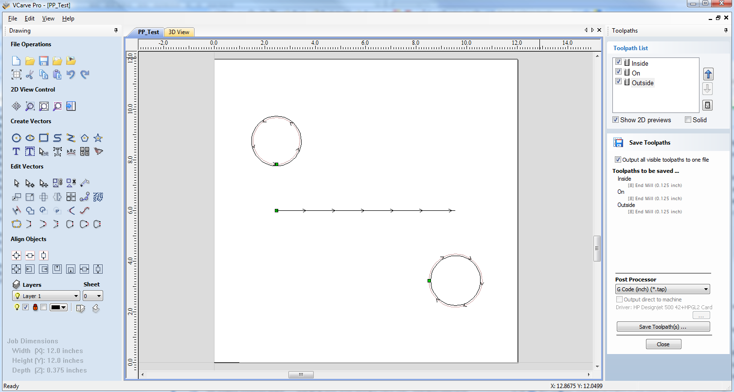
Speichern Sie einen Werkzeugpfad mit Ihrem Basis-Postprozessor und prüfen Sie ihn mit Ihrem bevorzugten Texteditor. Unten finden Sie ein Beispiel einer mit dem Postprozessor „G-Code Arcs (inch) (*.tap)“ ausgegebenen Testdatei. Das folgende Beispiel wird auf dem beliebten Editor Notepad++ angezeigt.
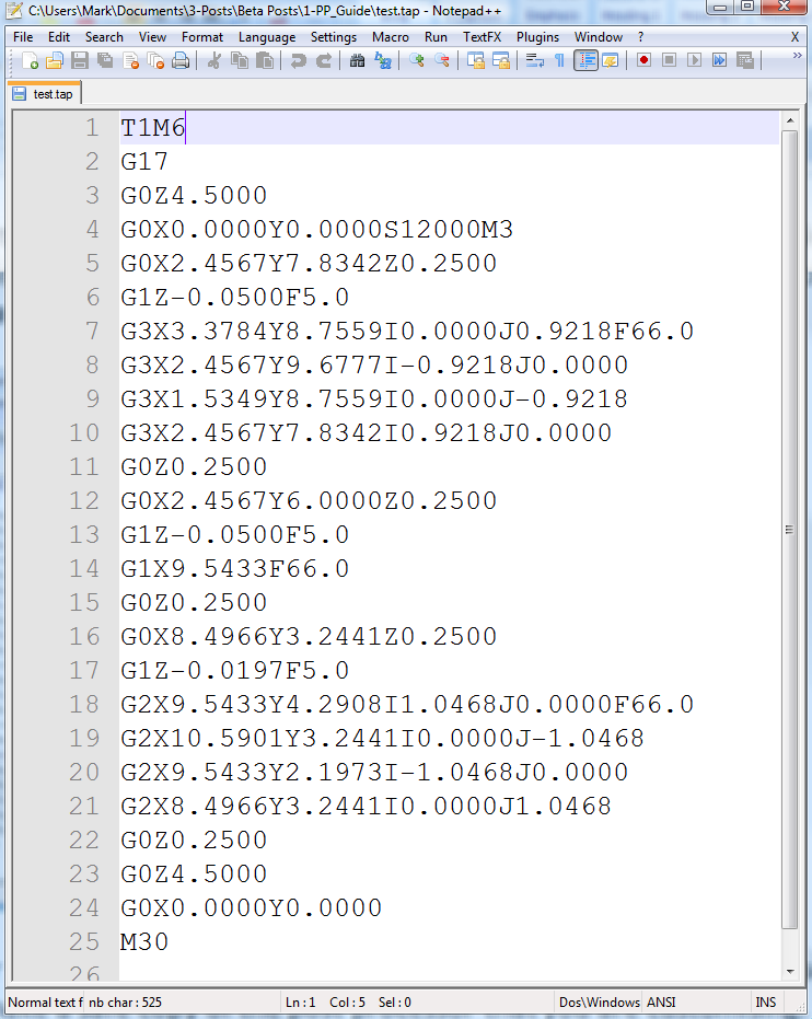
Für unser Beispiel fügen wir diesem Postprozessor einen Abschnitt für einen Werkzeugwechsel hinzu. Erstellen Sie zunächst eine Sicherheitskopie des Postprozessors, den Sie anpassen. Wenn Sie den zu bearbeitenden Postprozessor in einem Texteditor öffnen, sehen Sie die Textzeilen innerhalb des Postprozessor, welche die Ausgabe Ihrer Testdatei formatiert haben.
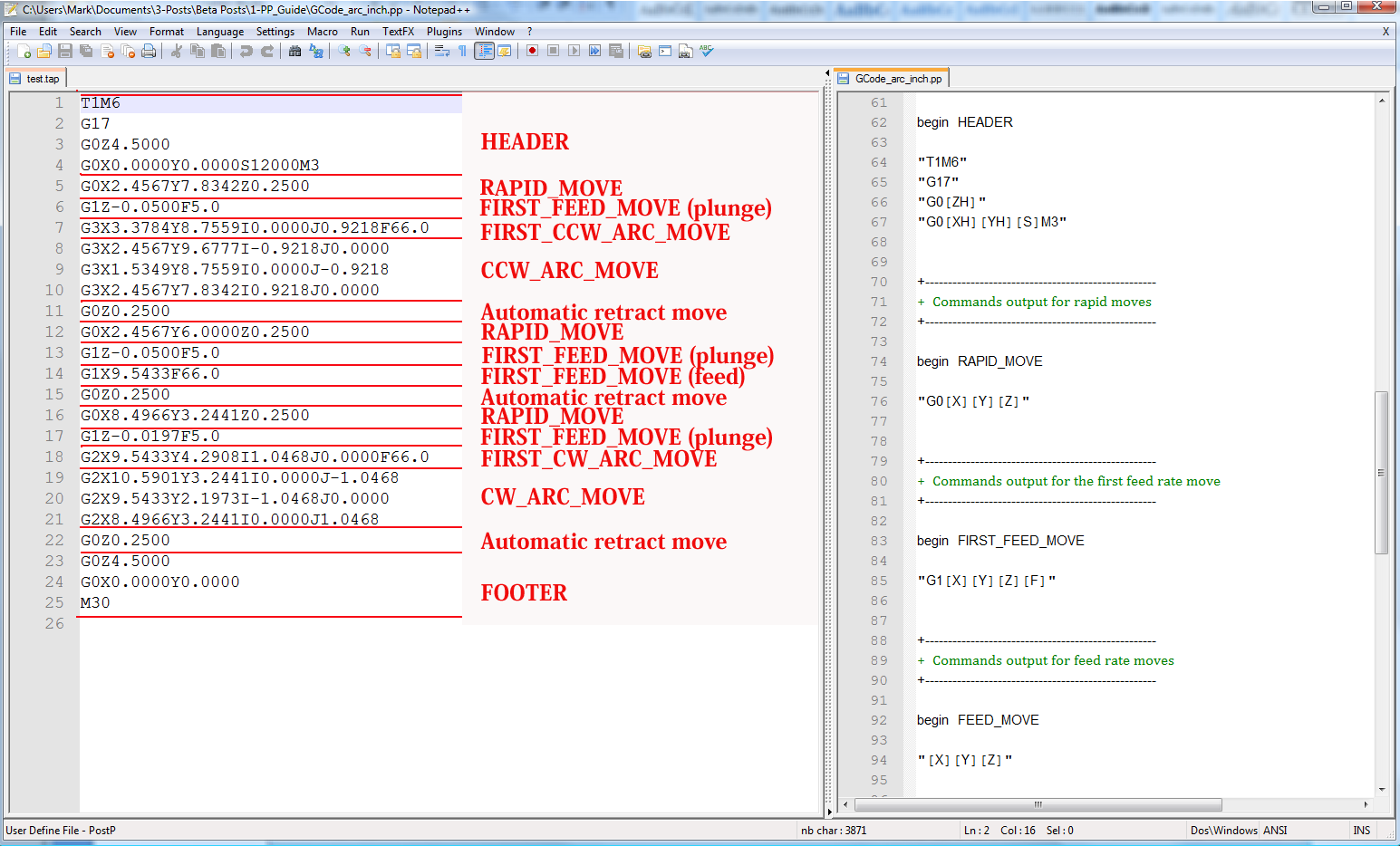
- Den Ordner PostP finden Sie über das Hauptmenü der Anwendung. Klicken Sie hierzu auf „Datei > Ordner mit Anwendungsdaten öffnen“.
Um dem Postprozessor einen Abschnitt für einen Werkzeugwechsel hinzuzufügen, ziehen Sie die Dokumentation für die Steuerung des Fräswerkzeugs (oder der Steuersoftware) heran. Für dieses Beispiel gehen wir davon aus, dass die benötigten Anweisungen für einen Werkzeugwechsel bei diesem speziellen Fräswerkzeug folgendermaßen lauten:
- M05 Anweisung, um die Spindel vor dem Werkzeugwechsel abzuschalten.
- M0 Anweisung, das aktive Werkzeug zum Werkzeughalter zurückzuführen.
- M06TTool_Number n Anweisung, das neue Werkzeug Tool_Number n auszuwählen
- G43HTool_Number n Anweisung an die Steuerung, für Werkzeug n den Versatz für die Werkzeuglänge zu verwenden
- Sxxx M03 Spindeldrehzahl auf xxx festlegen; Spindel einschalten (Drehung im Uhrzeigersinn).
Den Postprozessor mit Ihrem bevorzugten Texteditor bearbeiten.
Wenn Ihr Computer als Betriebssystem Windows Vista verwendet und die Benutzerzugriffskontrolle aktiviert ist, kopieren oder verschieben Sie den Postprozessor, den Sie bearbeiten, vom Ordner "PostP" in einen Ordner unterhalb Ihres Benutzerbereichs.
Bearbeiten Sie in der Datei zunächst den Bereich "Verlaufskommentare". Auf diese Weise erhalten sie einen Änderungsverlauf.
Bearbeiten Sie als nächstes den POST_NAME, um zu kennzeichnen, dass dieser Postprozessor Befehle für automatische Werkzeugwechsel (ATC) ausgibt. Der neue Post wird in der Liste der Postprozessoren als "G-Code ATC Arcs (inch)(*.tap)" angezeigt.
Fügen Sie dann einen Abschitt für Werkzeugwechsel mit den Anweisungen ein. Wo sich der neue Abschnitt innerhalb der Datei befindet, ist nicht von Bedeutung. Sinnvoll ist jedoch eine Position zwischen der Kopfzeile und den Abschnitten für schnelle Bewegungen.
Fügen Sie zu Beginn des neuen Abschnitts einige Kommentare hinzu (beginnend mit dem Zeichen "+"), um den Abschnitt zu beschreiben und die Datei als Ganzes einfacher lesbar zu machen. Geben Sie als nächstes die Zeile „begin TOOLCHANGE“ ein, um den Postprozessor anzuweisen, dass die folgenden Anweisungen bei jedem Werkzeugwechsel ausgegeben werden sollen (außer für die erste Werkzeugauswahl, hierfür befinden sich die Befehle in der Kopfzeile).
Geben Sie als nächsten Schritt die erforderlichen Anweisungen in doppelten Anführungszeichen ein. Das „[T]“ in der dritten und vierten Anweisungszeile unseres Beispiels wird bei der Verarbeitung der Datei durch die Werkzeugnummer ersetzt. Das „[S]“ in der fünften Zeile wird durch die Spindeldrehzahl für das Werkzeug ersetzt.
Speichern Sie schließlich die Änderungen an der Datei. Da Sie POST_NAME geändert haben, speichern Sie die Datei unter einem neuen Namen, beispielsweise "GCODE_ATC_Arcs_inch.pp".
Wenn Ihr Computer als Betriebssystem Windows 7 oder Windows Vista verwendet und die Benutzerzugriffskontrolle aktiviert ist, kopieren Sie die bearbeitete Datei zurück in den Ordner "PostP".
Wenn die Software funktioniert, starten Sie diese neu, um den Postprozessor zu testen.
Sollten in Ihrem Postprozessor Syntaxfehler vorliegen, wird beim Start der Software ein Fehler ähnlich der Abbildung unten angezeigt. Zudem wird der bearbeitete Postprozessor nicht in der Drop-down-Liste mit Postprozessor-Konfigurationsdateien angezeigt. Korrigieren Sie alle Fehler und starten Sie die Software neu.
Wenn beim Start der Software keine Fehler angezeigt werden, öffnen Sie Ihre Testdatei und speichern Sie einen oder mehrere Ihrer Test-Werkzeugpfade.
Wählen Sie den Postprozessor aus der Dropdown-Liste mit Postprozessor-Konfigurationen und wählen Sie die Schaltfläche "Werkzeugpfad(e) speichern".
Schauen Sie sich die Datei an, die Sie gerade in einem Texteditor gespeichert haben.
Wenn der Dateiinhalt einen korrekten Eindruck macht, testen Sie die Datei mit Ihrer Maschine.
Ergreifen Sie bitte alle erforderlichen Vorsichtsmaßnahmen, wenn Sie die Ausgabe erstmals über einen modifizierten Postprozessor betreiben.
Beispiel: Dateierweiterung ändern
Die Dateierweiterung, die der Postprozessor automatisch erstellt, kann mit einem Klick auf die Schaltfläche "Werkzeugpfad(e) speichern" im Dialogfeld "Speichern als" geändert werden.
Statt jedoch die Dateierweiterung jedes Mal zu ändern, ist es komfortabler, die durch den Postprozessor erstellte Dateierweiterung dauerhaft zu ändern.
Verfahren Sie hierzu wie folgt:
Erstellen Sie eine Sicherheitskopie des Postprozessors, den Sie bearbeiten möchten.
Die Konfigurationsdateien des Postprozessors befinden sich im Ordner "PostP" des Produktinstallationsordners und verwenden die Dateierweiterung ".PP". Für Aspire, Version 2, befindet sich der Ordner "PostP" üblicherweise unter: "C:\Program Files\Aspire V2.0\PostP". Je nach installiertem Produkt und abhängig davon, ob die Software an einem benutzerdefinierten Ort erstellt wurde, kann sich der Ordner "PostP" an einem anderen Ort befinden.
Bearbeiten Sie den Postprozessor mit Ihrem bevorzugten Texteditor.
Wenn Ihr Computer als Betriebssystem Microsoft Windows 7 oder Windows Vista verwendet und die Benutzerzugriffskontrolle aktiviert ist, kopieren oder verschieben Sie den Postprozessor, den Sie bearbeiten, vom Ordner "PostP" in einen Ordner unterhalb Ihres Benutzerbereichs.
Suchen Sie nach den beiden Zeilen in der Konfigurationsdatei des Postprozessors, die folgendermaßen beginnen:
POST_NAME =
FILE_EXTENSION =
und verändern sie diese entsprechend.
Wenn Sie beispielsweise die durch den Postprozessor "G Code ATC (inch)(*.tap)" erstellten Dateierweiterungen von ".tap" zu ".nc" ändern möchten, ändern Sie die Zeilen:
POST_NAME = "G Code ATC (inch) (*.tap)"
FILE_EXTENSION = "tap"
zu:
POST_NAME = "G Code ATC (inch) (*.nc)"
FILE_EXTENSION = "nc"
Speichern Sie die Änderungen an Ihrer Datei. Wenn Ihr Computer als Betriebssystem Windows 7 oder Windows Vista verwendet und die Benutzerzugriffskontrolle aktiviert ist, kopieren Sie die bearbeitete Datei zurück in den Ordner "PostP".
Wenn die Software funktioniert, starten Sie diese neu, um den Postprozessor zu testen. Sollten in Ihrem Postprozessor Syntaxfehler vorliegen, wird beim Start der Software ein Fehler ähnlich der Abbildung unten angezeigt. Zudem wird der bearbeitete Postprozessor nicht in der Drop-down-Liste mit Postprozessor-Konfigurationsdateien angezeigt. Korrigieren Sie alle Fehler und starten Sie die Software neu.
Wenn beim Start der Software keine Fehler angezeigt werden, öffnen Sie Ihre Testdatei und speichern Sie einen oder mehrere Ihrer Test-Werkzeugpfade.
Wählen Sie den Postprozessor aus der Dropdown-Liste mit Postprozessor-Konfigurationen und wählen Sie die Schaltfläche "Werkzeugpfad(e) speichern".
Schauen Sie sich die Datei an, die Sie gerade in einem Texteditor gespeichert haben.
Wenn der Dateiinhalt einen korrekten Eindruck macht, testen Sie die Datei mit Ihrer Maschine.
Ergreifen Sie bitte alle erforderlichen Vorsichtsmaßnahmen, wenn Sie die Ausgabe erstmals über einen modifizierten Postprozessor betreiben.
Tipps und Tricks
1. Erstellen Sie immer eine Sicherheitskopie des Postprozessors, den Sie bearbeiten, falls Sie noch einmal von Null beginnen müssen.
2. Sollten Sie einen Postprozessor mithilfe eines Textverarbeitungsprogramms wie Microsoft Word bearbeiten, speichern Sie die Datei unbedingt als reine Textdatei. In der Datei dürfen sich keine Formatierungsdaten befinden.
3. Wenn Sie Postprozessoren auf einem Computer bearbeiten, der als Betriebssystem Microsoft Windows 7 oder Windows Vista verwendet, bearbeieten Sie die Dateien nicht direkt im Ordner "Program Files\Product folder\PostP". Bearbeiten Sie die Datei immer in Ihrem Benutzerbereich und kopieren sie die bearbeitete Datei in den Ordner "Program Files\Product folder\PostP".
4. Kommentieren Sie Änderungen. Ein Kommentar ist der Text, der auf die Zeichen + oder | folgt. Das Programm reagiert nicht auf Kommentare. Sie sind jedoch bei der Dokumentierung der durchgeführten Änderungen hilfreich und stellen diese für die Zukunft verständlich dar.
5. Alle Anweisungszeilen müssen von Anführungszeichen umschlossen sein.
6. Verwenden Sie nach Möglichkeit einen Texteditor, der Zeilen nummeriert. Dies erleichtert bei Fehlern in der Datei die Fehlersuche im Postprozessor. Das Programm prüft beim Start die Postprozessoren im Ordner "PostP". Bei Syntaxfehlern in der Datei wird eine Fehlermeldung mit der Zeilennummer herausgegeben, in welcher der Fehler als erstes erkannt wurde.
7. Wenn Sie einen Postprozessor erfolgreich bearbeitet haben, erstellen Sie eine Sicherungskopie. Wenn Sie eine neuere Version ihres verwendeten Vectric-Produkts installieren, kopieren sie Ihren angepassten Postprozessor in den Ordner "PostP" der neuen Softwareversion. Wählen Sie außerdem den angepassten Postprozessor aus, wenn Sie den ersten Werkzeugpfad speichern (für Folgeaktionen merkt sich die Software Ihre Auswahl).
8. Wenn Sie eine andere Version der Software installieren oder ein Versionsupgrade der Software durchführen, kopieren Sie die Sicherungskopien Ihrer bearbeiteten Postprozessoren in den Ordner "PostP" der neuen Version. Achten Sie darauf, für die erste Datei in der neuen Softwareversion den richtigen Postprozessor auszuwählen.
9. Greifen Sie bei neueren Versionen der Software (V5.5 und höher) aus der Anwendung auf die Postprozessoren zu. Klicken sie hierzu auf den Ordner "File > Open Application Data Folder\PostP".
10. Sie können eine angepasste Liste der Postprozessoren erstellen. Kopieren Sie hierzu ausschließlich die benötigten Postprozessoren in den Ordner "File > Open Application Data Folder\My_PostP". Sollte im Ordner "My_PostP" eine Datei mit der Erweiterung .pp existieren, werden in der Dropdown-Liste nur die Postprozessoren im Ordner "My_PostP" angezeigt.